Visualization
- ERF currently generates plotfile in the native AMReX format or as NetCDF files; see
Plotfiles for how to set the plotfile options.
There are several visualization tools that can be used for AMReX plotfiles, specifically ParaView, VisIt and yt.
In addition, a new tool called “pltview” is available at https://github.com/wang1202/pltview; this is a lightweight X11 viewer for AMReX plotfiles. See the plotview README for more details on how to download and install pltview.
If NetCDF output is preferred, one suggestion is to write the plotfiles in the native AMReX format for efficient I/O performance, then to convert the plotfiles to NetCDF files using the executable you can build in Exec/Tools.
ParaView
The open source visualization package ParaView v5.10 and later can be used to view ERF plotfiles with and without terrain. You can download the paraview executable at https://www.paraview.org/.
To open a plotfile
Run ParaView v5.10, then select “File” \(\rightarrow\) “Open”.
Navigate to your run directory, and select either a single plotfile or a set of plotfiles. Open multiple plotfile at once by selecting
plt..Paraview will load the plotfiles as a time series. ParaView will ask you about the file type – choose “AMReX/BoxLib Grid Reader”.If you have run the ERF executable with terrain-fitted coordinates, then the mapped grid information will be stored as nodal data. Choose the “point data” called “nu”, then click on “Warp by Vector” which can be found via Filters–>Alphabetical. This will then plot data onto the mapped grid locations.
Under the “Cell Arrays” field, select a variable (e.g., “x_velocity”) and click “Apply”. Note that the default number of refinement levels loaded and visualized is 1. Change to the required number of AMR level before clicking “Apply”.
For “Representation” select “Surface”.
For “Coloring” select the variable you chose above.
To add planes, near the top left you will see a cube icon with a green plane slicing through it. If you hover your mouse over it, it will say “Slice”. Click that button.
You can play with the Plane Parameters to define a plane of data to view, as shown in 5.
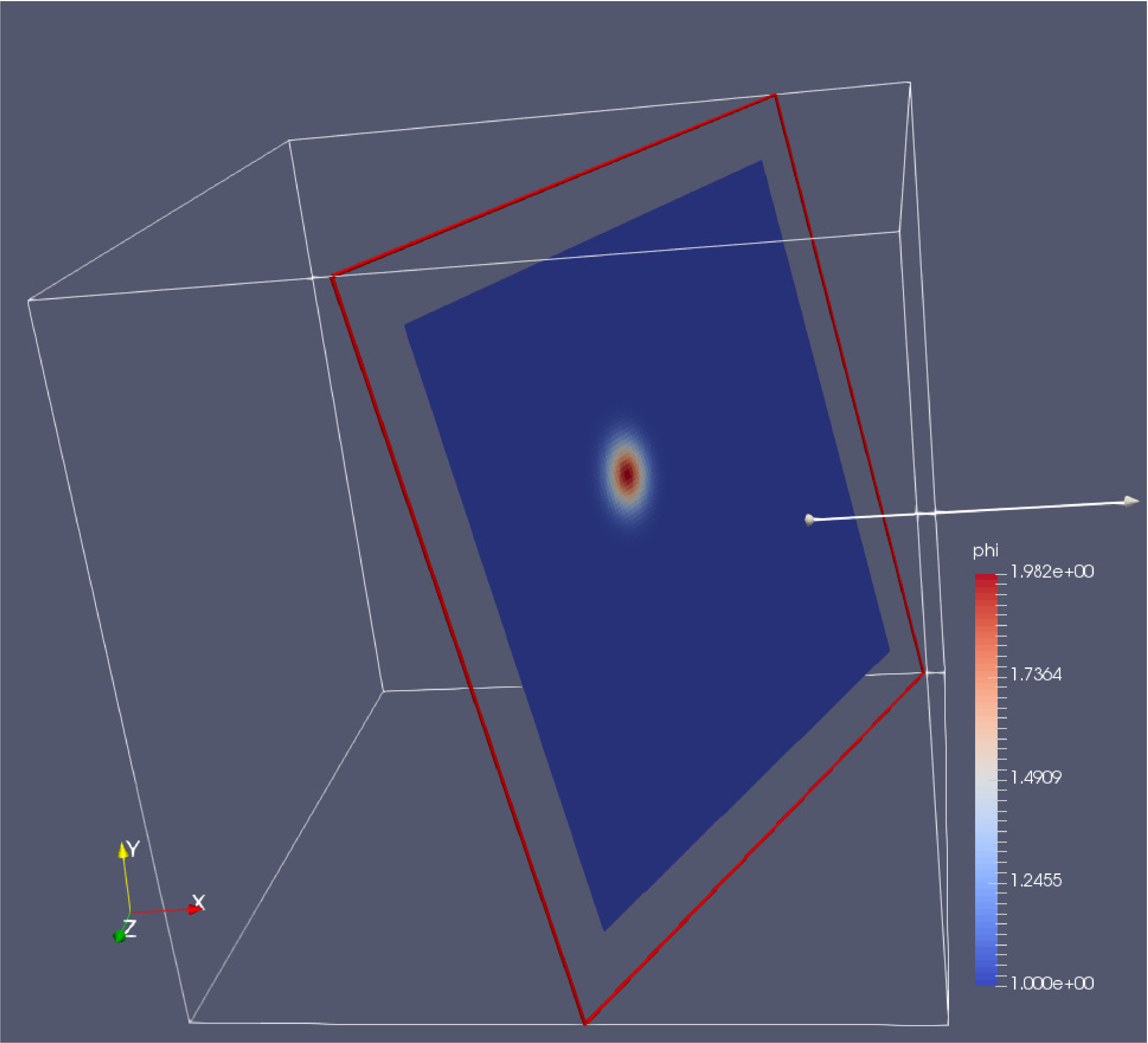
5 : Plotfile image generated with ParaView
VisIt
AMReX data can also be visualized by VisIt, an open source visualization and analysis software. To follow along with this example, first build and run the first heat equation tutorial code.
Next, download VisIt from https://visit-dav.github.io/visit-website/ and install. To open a single plotfile, run VisIt, then select “File” \(\rightarrow\) “Open file …”, then select the Header file associated the the plotfile of interest (e.g., plt00000/Header). Assuming you ran the simulation in 2D, here are instructions for making a simple plot:
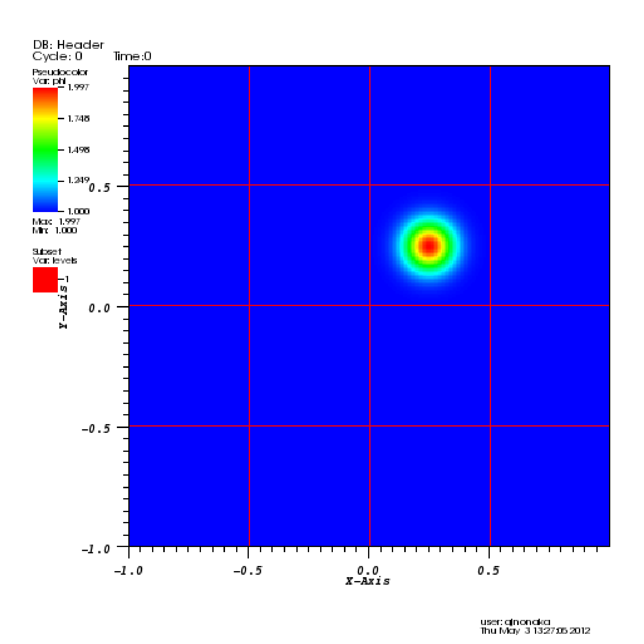
To view the data, select “Add” \(\rightarrow\) “Pseudocolor” \(\rightarrow\) “phi”, and then select “Draw”.
To view the grid structure (not particularly interesting yet, but when we add AMR it will be), select “Add” \(\rightarrow\) “Subset” \(\rightarrow\) “levels”. Then double-click the text “Subset - levels”, enable the “Wireframe” option, select “Apply”, select “Dismiss”, and then select “Draw”.
To save the image, select “File” \(\rightarrow\) “Set save options”, then customize the image format to your liking, then click “Save”.
Your image should look similar to the left side of 13.
|
|
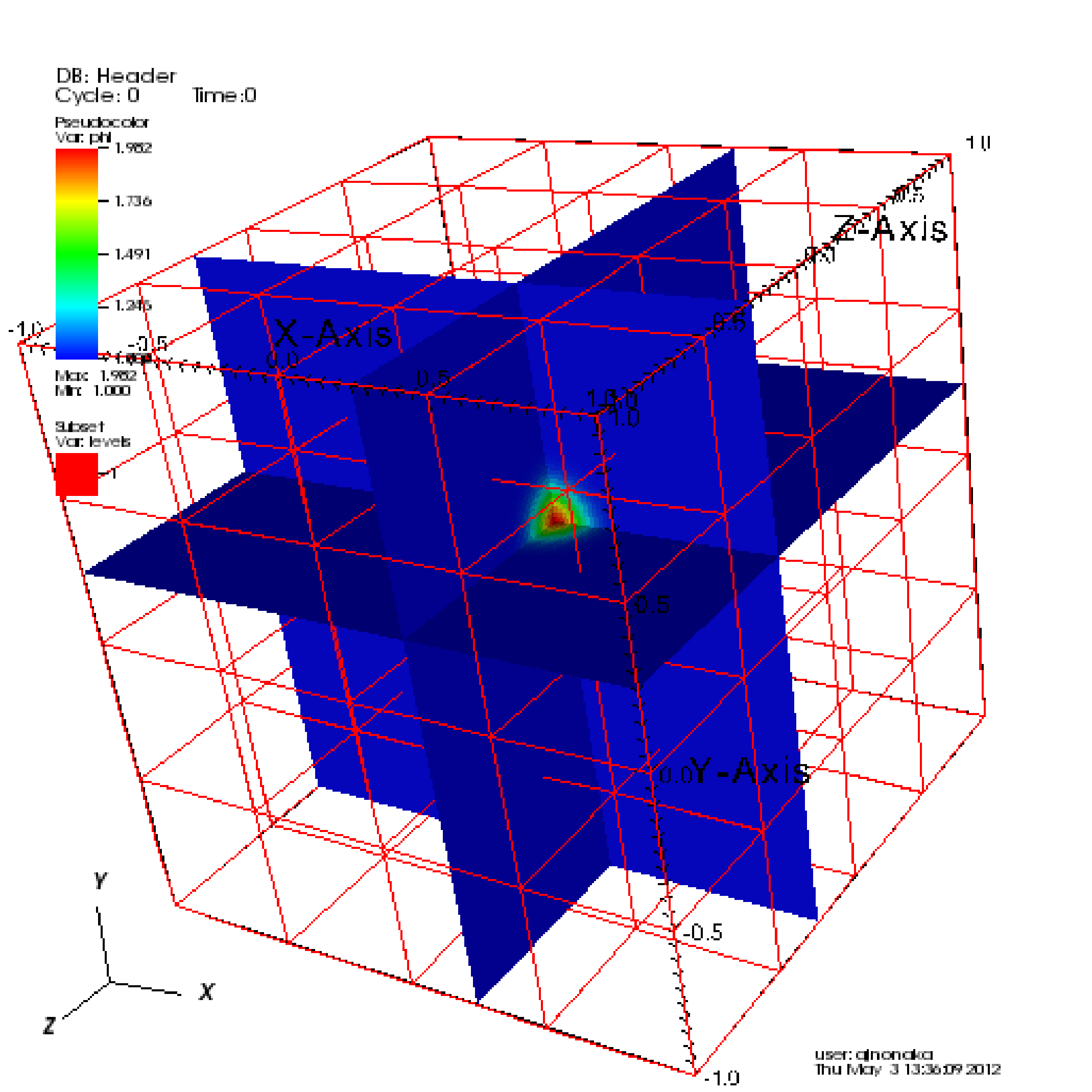
In 3D, you must apply the “Operators” \(\rightarrow\) “Slicing”
\(\rightarrow\) “ThreeSlice”, with the “ThreeSlice operator attribute” set
to x=0.25, y=0.25, and z=0.25. You can left-click and drag over the
image to rotate the image to generate something similar to right side of
13.
To make a movie, you must first create a text file named movie.visit with a
list of the Header files for the individual frames. This can most easily be
done using the command:
~/amrex/Tutorials/Basic/HeatEquation_EX1_C> ls -1 plt*/Header | tee movie.visit
plt00000/Header
plt01000/Header
plt02000/Header
plt03000/Header
plt04000/Header
plt05000/Header
plt06000/Header
plt07000/Header
plt08000/Header
plt09000/Header
plt10000/Header
The next step is to run VisIt, select “File” \(\rightarrow\) “Open file…”, then select movie.visit. Create an image to your liking and press the “play” button on the VCR-like control panel to preview all the frames. To save the movie, choose “File” \(\rightarrow\) “Save movie …”, and follow the on-screen instructions.
Caveat:
The Visit reader determines “Cycle” from the name of the plotfile (directory), specifically from the integer that follows the string “plt” in the plotfile name.
So … if you call it plt00100 or myplt00100 or this_is_my_plt00100 then it will correctly recognize and print Cycle: 100.
If you call it plt00100_old it will also correctly recognize and print Cycle: 100
But, if you do not have “plt” followed immediately by the number, e.g. you name it pltx00100, then VisIt will not be able to correctly recognize and print the value for “Cycle”. (It will still read and display the data itself.)
yt
yt, an open source Python package available at https://yt-project.org/, can be used for analyzing and visualizing mesh and particle data generated by AMReX codes. Some of the AMReX developers are also yt project members. Below we describe how to use on both a local workstation, as well as at the NERSC HPC facility for high-throughput visualization of large data sets.
We also note that there is active development of an xarray-like interface for AMReX simulation data via yt; see the xamr docs for more details.
Note - AMReX datasets require yt version 3.4 or greater.
Using on a local workstation
Running yt on a local system generally provides good interactivity, but limited performance. Consequently, this configuration is best when doing exploratory visualization (e.g., experimenting with camera angles, lighting, and color schemes) of small data sets.
To use yt on an AMReX plot file, first start a Jupyter notebook or an IPython
kernel, and import the yt module:
In [1]: import yt

In [2]: print(yt.__version__)
3.4-dev
Next, load a plot file; in this example we use a plot file from the Nyx cosmology application:
In [3]: ds = yt.load("plt00401")
yt : [INFO     ] 2017-05-23 10:03:56,182 Parameters: current_time              = 0.00605694344696544
yt : [INFO     ] 2017-05-23 10:03:56,182 Parameters: domain_dimensions         = [128 128 128]
yt : [INFO     ] 2017-05-23 10:03:56,182 Parameters: domain_left_edge          = [ 0.  0.  0.]
yt : [INFO     ] 2017-05-23 10:03:56,183 Parameters: domain_right_edge         = [ 14.24501  14.24501  14.24501]

In [4]: ds.field_list
Out[4]:
[('DM', 'particle_mass'),
 ('DM', 'particle_position_x'),
 ('DM', 'particle_position_y'),
 ('DM', 'particle_position_z'),
 ('DM', 'particle_velocity_x'),
 ('DM', 'particle_velocity_y'),
 ('DM', 'particle_velocity_z'),
 ('all', 'particle_mass'),
 ('all', 'particle_position_x'),
 ('all', 'particle_position_y'),
 ('all', 'particle_position_z'),
 ('all', 'particle_velocity_x'),
 ('all', 'particle_velocity_y'),
 ('all', 'particle_velocity_z'),
 ('boxlib', 'density'),
 ('boxlib', 'particle_mass_density')]
From here one can make slice plots, 3-D volume renderings, etc. An example of the slice plot feature is shown below:
In [9]: slc = yt.SlicePlot(ds, "z", "density")
yt : [INFO     ] 2017-05-23 10:08:25,358 xlim = 0.000000 14.245010
yt : [INFO     ] 2017-05-23 10:08:25,358 ylim = 0.000000 14.245010
yt : [INFO     ] 2017-05-23 10:08:25,359 xlim = 0.000000 14.245010
yt : [INFO     ] 2017-05-23 10:08:25,359 ylim = 0.000000 14.245010

In [10]: slc.show()

In [11]: slc.save()
yt : [INFO     ] 2017-05-23 10:08:34,021 Saving plot plt00401_Slice_z_density.png
Out[11]: ['plt00401_Slice_z_density.png']
The resulting image is 6. One can also make volume renderings with ; an example is show below:
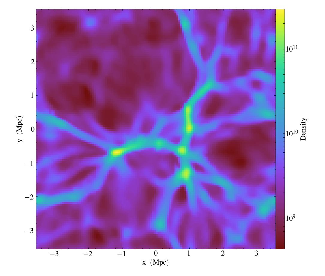
6 : Slice plot of \(128^3\) Nyx simulation using yt.
In [12]: sc = yt.create_scene(ds, field="density", lens_type="perspective")

In [13]: source = sc[0]

In [14]: source.tfh.set_bounds((1e8, 1e15))

In [15]: source.tfh.set_log(True)

In [16]: source.tfh.grey_opacity = True

In [17]: sc.show()
<Scene Object>:
Sources:
    source_00: <Volume Source>:YTRegion (plt00401): , center=[  1.09888770e+25   1.09888770e+25   1.09888770e+25] cm, left_edge=[ 0.  0.  0.] cm, right_edge=[  2.19777540e+25   2.19777540e+25   2.19777540e+25] cm transfer_function:None
Camera:
    <Camera Object>:
    position:[ 14.24501  14.24501  14.24501] code_length
    focus:[ 7.122505  7.122505  7.122505] code_length
    north_vector:[ 0.81649658 -0.40824829 -0.40824829]
    width:[ 21.367515  21.367515  21.367515] code_length
    light:None
    resolution:(512, 512)
Lens: <Lens Object>:
    lens_type:perspective
    viewpoint:[ 0.95423473  0.95423473  0.95423473] code_length

In [19]: sc.save()
yt : [INFO     ] 2017-05-23 10:15:07,825 Rendering scene (Can take a while).
yt : [INFO     ] 2017-05-23 10:15:07,825 Creating volume
yt : [INFO     ] 2017-05-23 10:15:07,996 Creating transfer function
yt : [INFO     ] 2017-05-23 10:15:07,997 Calculating data bounds. This may take a while.
Set the TransferFunctionHelper.bounds to avoid this.
yt : [INFO     ] 2017-05-23 10:15:16,471 Saving render plt00401_Render_density.png
The output of this is 7.