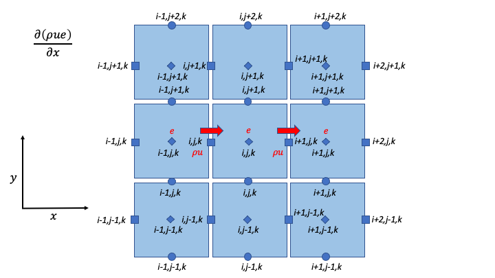
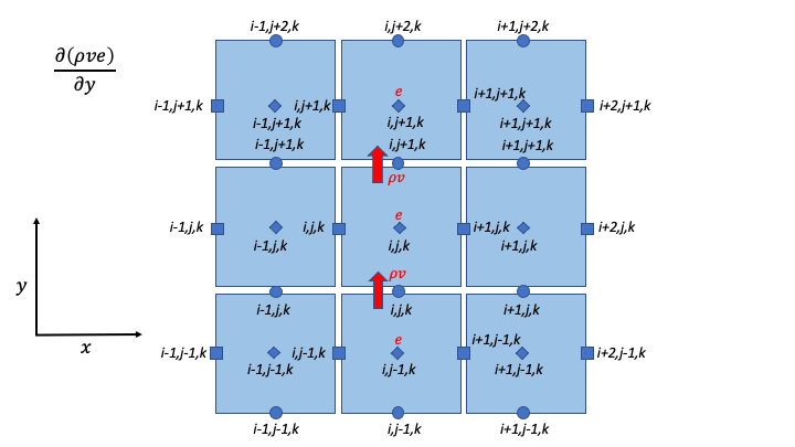
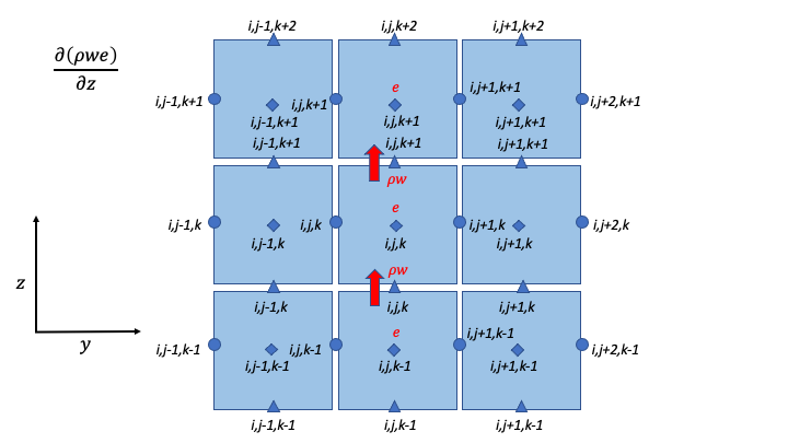
Advection Contribution to DNS/LES
U Momentum
\[\begin{split}\begin{align}
\left( \rho u \right)_{i,j,k}^{n + 1} & = \left( \rho u \right)_{i,j,k}^{n} - \\
\Delta t & \left\{ \frac{1}{2\Delta x}\ \left\lbrack \left( \left( \rho u \right)_{i + 1,j,k}^{n} + \left( \rho u \right)_{i,j,k}^{n} \right)u_{i + \frac{1}{2},j,k}^{n} - \left( \left( \rho u \right)_{i,j,k}^{n} + \left( \rho u \right)_{i - 1,j,k}^{n} \right)u_{i - \frac{1}{2},j,k}^{n} \right\rbrack \right. \\
& + \frac{1}{2\Delta y} \left\lbrack \left( \left( \rho v \right)_{i,j + 1,k}^{n} + \left( \rho v \right)_{i - 1,j + 1,k}^{n} \right)u_{i,j + \frac{1}{2},k}^{n} - \left( \left( \rho v \right)_{i,j,k}^{n} + \left( \rho v \right)_{i - 1,j,k}^{n} \right)u_{i,j - \frac{1}{2},k}^{n} \right\rbrack \\
& + \left. \frac{1}{2\Delta z} \left\lbrack \left( \left( \rho w \right)_{i,j,k + 1}^{n} + \left( \rho w \right)_{i - 1,j,k + 1}^{n} \right)u_{i,j,k + \frac{1}{2}}^{n} - \left( \left( \rho w \right)_{i,j,k}^{n} + \left( \rho w \right)_{i - 1,j,k}^{n} \right)u_{i,j,k - \frac{1}{2}}^{n} \right\rbrack \right\} \\
& - \frac{\Delta t}{\Delta x}\left\lbrack p_{i,\ j,\ k}^{n} - p_{i - 1,\ j,\ k}^{n} \right\rbrack \\
\end{align}\end{split}\]
Contributions from different directions
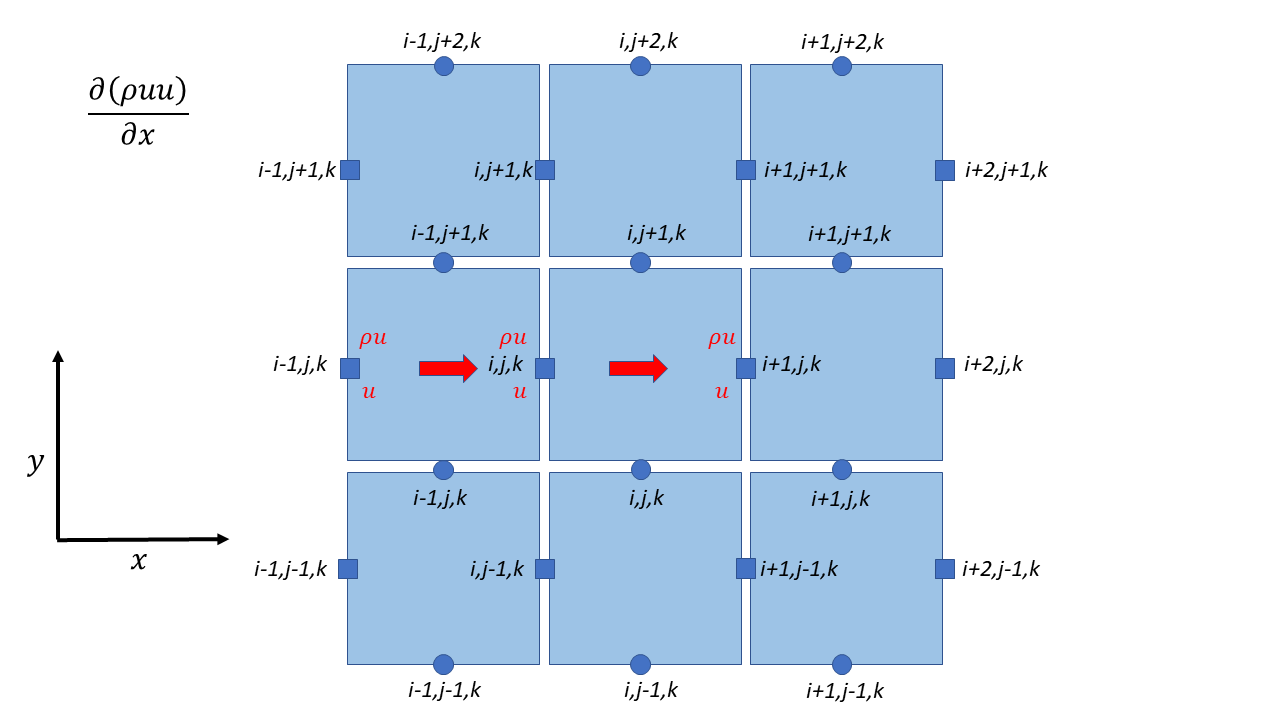
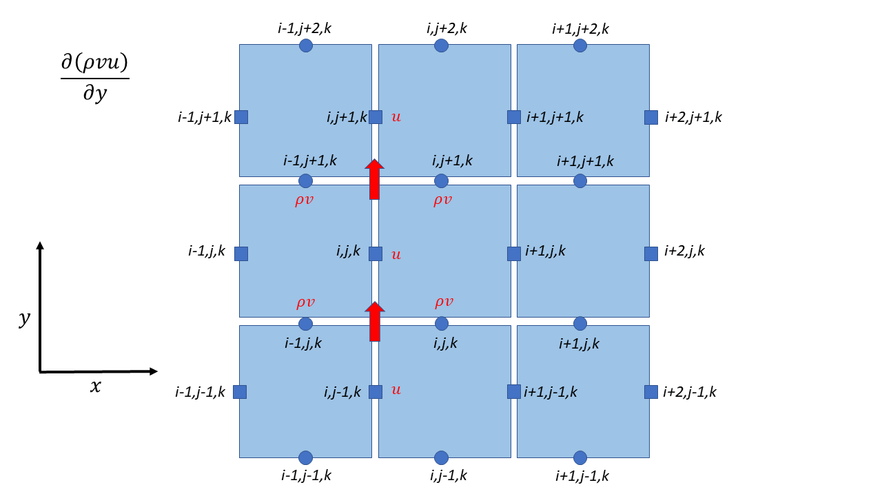
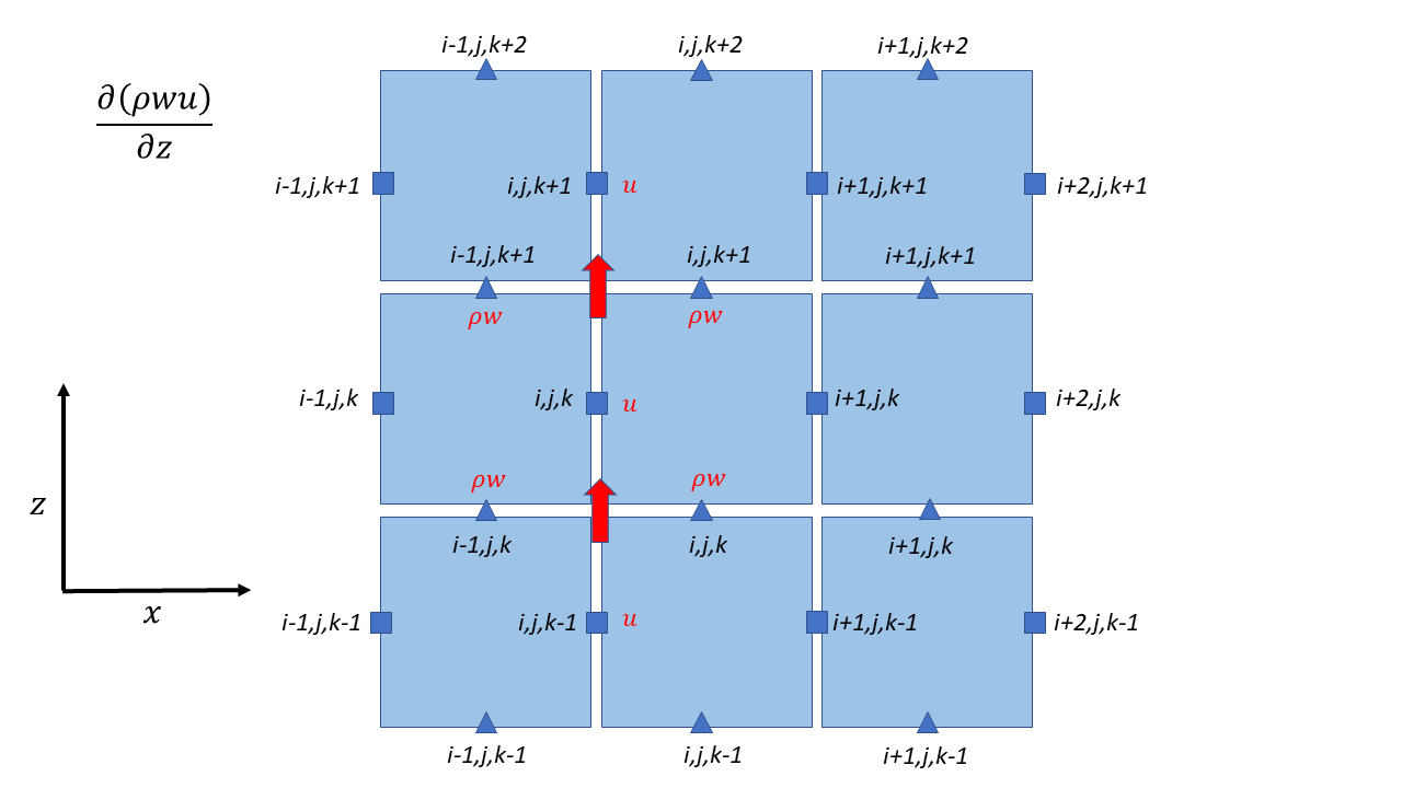
V Momentum
\[\begin{split}\begin{align}
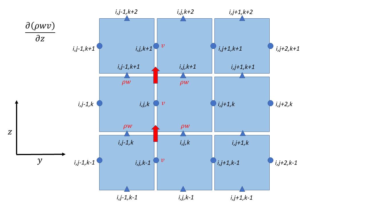
\left( \rho v \right)_{i,j,k}^{n + 1} & = \left( \rho v \right)_{i,j,k}^{n} - \\
\Delta t & \left\{ \frac{1}{2\Delta x}\ \left\lbrack \left( \left( \rho u \right)_{i + 1,j,k}^{n} + \left( \rho u \right)_{i + 1,j - 1,k}^{n} \right)v_{i + \frac{1}{2},j,k}^{n} - \left( \left( \rho u \right)_{i,j,k}^{n} + \left( \rho u \right)_{i,j - 1,k}^{n} \right)v_{i - \frac{1}{2},j,k}^{n} \right\rbrack \right. \\
& + \frac{1}{2\Delta y} \left\lbrack \left( \left( \rho v \right)_{i,j + 1,k}^{n} + \left( \rho v \right)_{i,j,k}^{n} \right)v_{i,j + \frac{1}{2},k}^{n} - \left( \left( \rho v \right)_{i,j,k}^{n} + \left( \rho v \right)_{i,j - 1,k}^{n} \right)v_{i,j - \frac{1}{2},k}^{n} \right\rbrack \\
& + \left. \ \frac{1}{2\Delta z} \left\lbrack \left( \left( \rho w \right)_{i,j,k + 1}^{n} + \left( \rho w \right)_{i,j - 1,k + 1}^{n} \right)v_{i,j,k + \frac{1}{2}}^{n} - \left( \left( \rho w \right)_{i,j,k}^{n} + \left( \rho w \right)_{i,j - 1,k}^{n} \right)v_{i,j,k - \frac{1}{2}}^{n} \right\rbrack \right\} \\
& - \frac{\Delta t}{\Delta y}\left\lbrack p_{i,j,\ k}^{n} - p_{i,\ j - 1,\ k}^{n} \right\rbrack \\
\end{align}\end{split}\]
Contributions from different directions
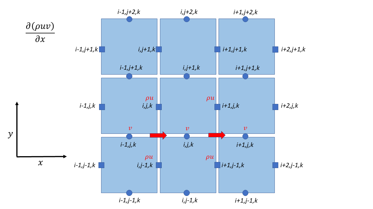
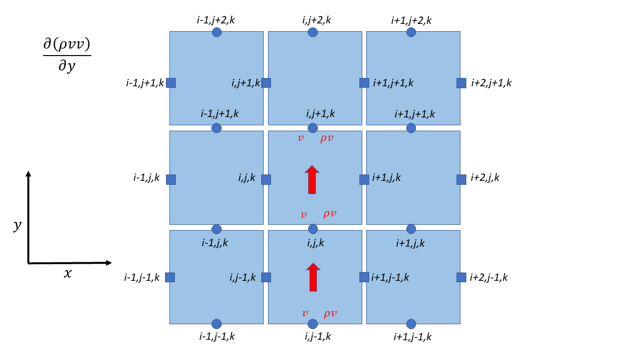
W Momentum
\[\begin{split}\begin{align}
\left( \rho w \right)_{i,j,k}^{n + 1} & = \left( \rho w \right)_{i,j,k}^{n} - \\
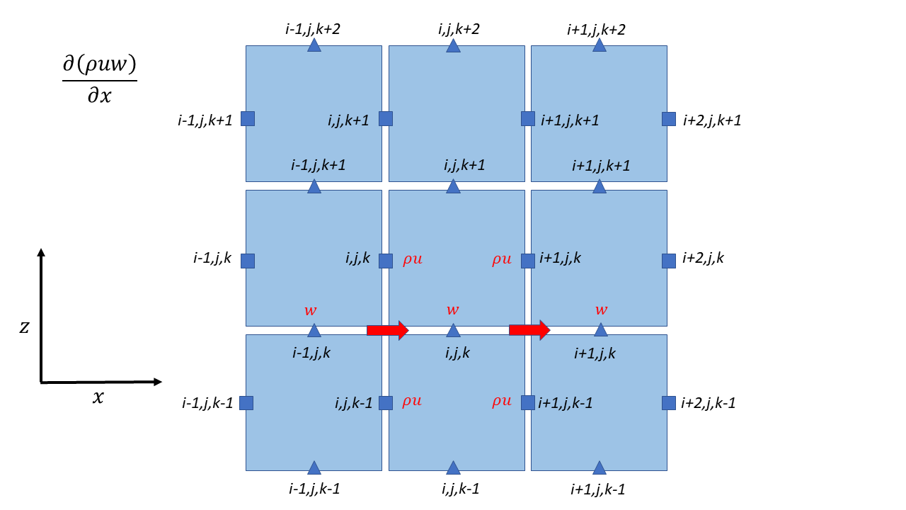
\Delta t & \left\{ \frac{1}{2\Delta x}\ \left\lbrack \left( \left( \rho u \right)_{i + 1,j,k}^{n} + \left( \rho u \right)_{i + 1,j,k - 1}^{n} \right)w_{i + \frac{1}{2},j,k}^{n} - \left( \left( \rho u \right)_{i,j,k}^{n} + \left( \rho u \right)_{i,j,k - 1}^{n} \right)w_{i - \frac{1}{2},j,k}^{n} \right\rbrack \right. \\
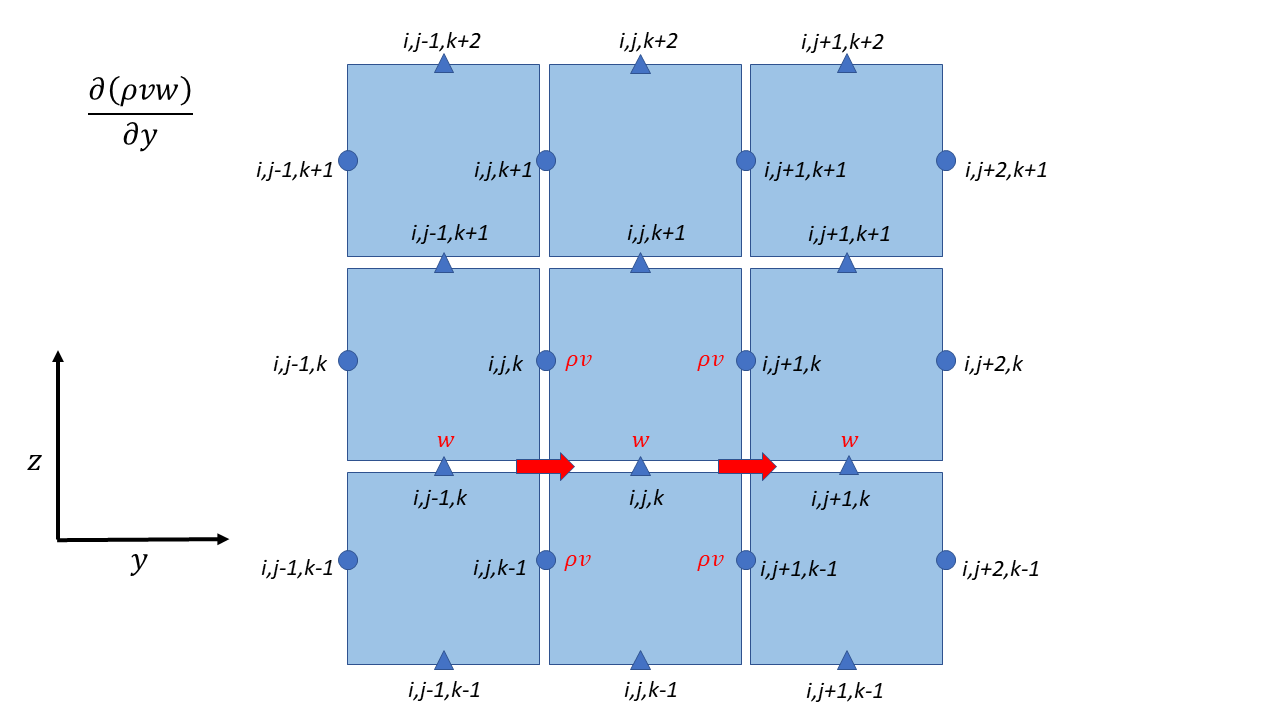
& + \frac{1}{2\Delta y} \left\lbrack \left( \left( \rho v \right)_{i,j + 1,k}^{n} + \left( \rho v \right)_{i,j + 1,k - 1}^{n} \right)w_{i,j + \frac{1}{2},k}^{n} - \left( \left( \rho v \right)_{i,j,k}^{n} + \left( \rho v \right)_{i,j,k - 1}^{n} \right)w_{i,j - \frac{1}{2},k}^{n} \right\rbrack \\
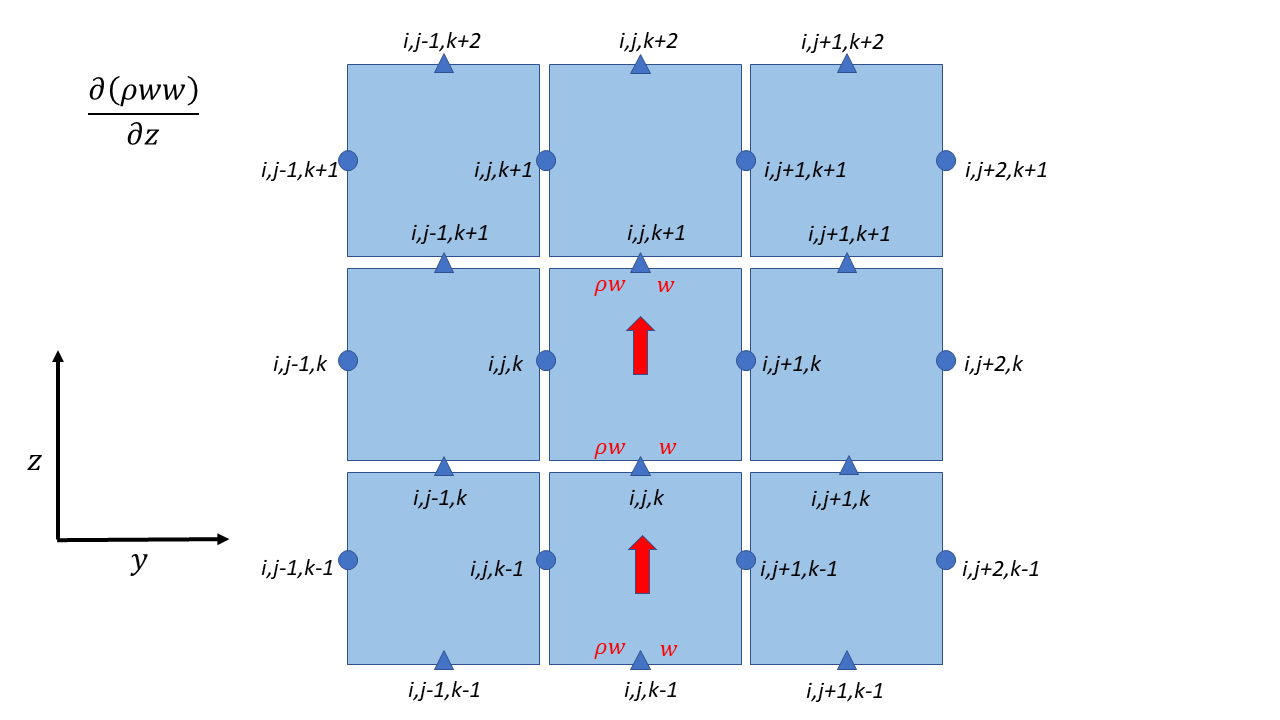
& + \left. \ \frac{1}{2\Delta z} \left\lbrack \left( \left( \rho w \right)_{i,j,k + 1}^{n} + \left( \rho w \right)_{i,j,k}^{n} \right)w_{i,j,k + \frac{1}{2}}^{n} - \left( \left( \rho w \right)_{i,j,k}^{n} + \left( \rho w \right)_{i,j,k - 1}^{n} \right)w_{i,j,k - \frac{1}{2}}^{n} \right\rbrack \right\} \\
& - \frac{\Delta t}{\Delta z}\left\lbrack p_{i,\ j,\ k}^{n} - p_{i,\ j,\ \ k - 1}^{n} \right\rbrack\ + \ \Delta t \left\lbrack \rho_{i,j,k - \ \frac{1}{2}}^{n} \right\rbrack g \\
\end{align}\end{split}\]
Contributions from different directions
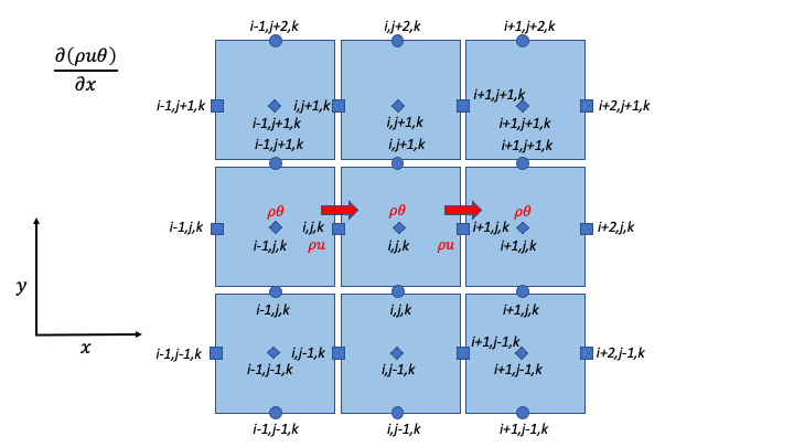
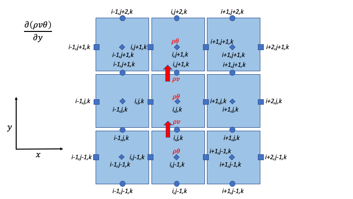
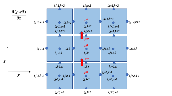
Potential Temperature Advection
\[\begin{split}\begin{align}
\left( \rho \theta \right)_{i,j,k}^{n + 1} = \left( \rho \theta \right)_{i,j,k}^{n} -
\Delta t & \left\{ \frac{1}{\Delta x}\ \left\lbrack \left( \rho u \right)_{i + 1,j,k}^{n} \theta_{i + \frac{1}{2},j,k}^{n} - \left( \rho u \right)_{i,j,k}^{n} \theta_{i - \frac{1}{2},j,k}^{n} \right\rbrack \right. \\
& + \frac{1}{\Delta y} \left\lbrack \left( \rho v \right)_{i,j + 1,k}^{n} \theta_{i,j + \frac{1}{2},k}^{n} - \left( \rho v \right)_{i,j,k}^{n} \theta_{i,j - \frac{1}{2},k}^{n} \right\rbrack \\
& + \left. \frac{1}{\Delta z} \left\lbrack \left( \rho w \right)_{i,j,k + 1}^{n} \theta_{i,j,k + \frac{1}{2}}^{n} - \left( \rho w \right)_{i,j,k}^{n} \theta_{i,j,k - \frac{1}{2}}^{n} \right\rbrack \right\} \\
\end{align}\end{split}\]
Contributions from different directions
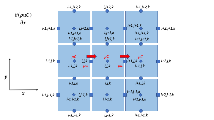
Scalar Advection
\[\begin{split}\begin{align}
\left( \rho C \right)_{i,j,k}^{n + 1} = \left( \rho C \right)_{i,j,k}^{n} -
\Delta t & \left\{ \frac{1}{\Delta x}\ \left\lbrack \left( \rho u \right)_{i + 1,j,k}^{n} C_{i + \frac{1}{2},j,k}^{n} - \left( \rho u \right)_{i,j,k}^{n} C_{i - \frac{1}{2},j,k}^{n} \right\rbrack \right. \\
& + \frac{1}{\Delta y} \left\lbrack \left( \rho v \right)_{i,j + 1,k}^{n} C_{i,j + \frac{1}{2},k}^{n} - \left( \rho v \right)_{i,j,k}^{n} C_{i,j - \frac{1}{2},k}^{n} \right\rbrack \\
& + \left. \frac{1}{\Delta z} \left\lbrack \left( \rho w \right)_{i,j,k + 1}^{n} C_{i,j,k + \frac{1}{2}}^{n} - \left( \rho w \right)_{i,j,k}^{n} C_{i,j,k - \frac{1}{2}}^{n} \right\rbrack \right\} \\
\end{align}\end{split}\]
Contributions from different directions

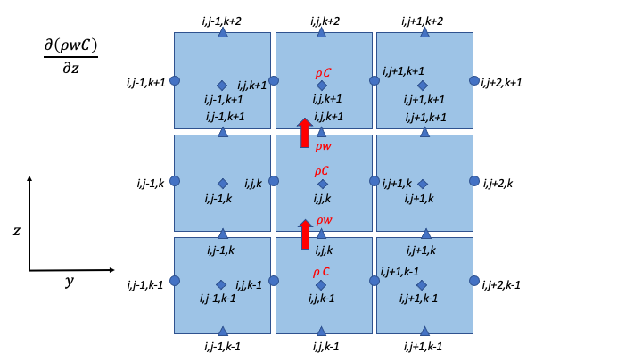
Scalar-advection field interface
ERF evaluates cell-centered scalar advection by reconstructing the primitive
scalar to each cell face, multiplying the reconstructed value by the
time-averaged mass flux through that face, and taking the finite-volume
divergence of the resulting scalar fluxes.
For the regular-grid and terrain-following scalar operator, the mapped
divergence has the form
\[\left.\frac{\partial (\rho C)}{\partial t}\right|_{\mathrm{adv}}
=
-\frac{m_x m_y}{J}
\left(
\frac{\partial F_x}{\partial x}
+
\frac{\partial F_y}{\partial y}
+
\frac{\partial F_z}{\partial z}
\right),\]
where \(J\) is the metric Jacobian, \(m_x\) and \(m_y\) are the
cell-centered map factors, and each \(F_d\) is the time-averaged mass flux
in direction \(d\) multiplied by the reconstructed scalar value on that
face.
The scalar-advection implementation treats the scalar input field, face-flux
storage, and output tendency as independent component views. ERF’s native
state adapter maps the model’s primitive-scalar layout onto those views, but
the numerical reconstruction and divergence operators do not require the
scalar to occupy a native conserved-state component. This separation allows
the same regular scalar-advection implementation to be reused by future
cell-centered scalar fields without first staging those fields into the
native conserved state.
This is an implementation interface rather than a new runtime option. It does
not change the available advection schemes, their configured inputs, or the
numerical treatment of ERF’s existing scalar state. This change does not add
an auxiliary tracer. Embedded-boundary scalar reconstruction and cut-cell
divergence retain their specialized EB implementation.
Diagnostic Variables
\[p_{i, j, k}^n = (\rho_{i, j, k}^n R_d \theta_{i, j, k}^n / p_0^{R_d / c_p} )^\gamma\]
\[T_{i, j, k}^n = \frac{p_{i, j, k}^n}{ \rho_{i, j, k}^n R_d}\]
Here \(\rho_{i, j, k}^n, T_{i, j, k}^n, \theta_{i, j, k}^n\), and \(p_{i, j, k}^n\) are the density, temperature, potential temperature and pressure, respectively;
these variables are all defined at cell centers of cell indexed by \((i, j, k)\) and at time level \(n\).
\(R_d\) and \(c_p\) are the gas constant and specific heat capacity for dry air respectively,
and \(\gamma = c_p / (c_p - R_d)\) . \(p_0\) is a reference value for pressure.
Differencing of Different Orders
Interpolation Methods
The midpoint values given above \(q_{m - \frac{1}{2}}\), where \(q\) may be \([u, v, w, \theta, C]\), \(m = i, j, k\), \(U_d = [u, v, w]\) for \([x, y, z]\) directions respectively, the following interpolation schemes are available:
\[\begin{split}\begin{array}{lll}
\left. q_{m - \frac{1}{2}} \right|^{2nd} = \frac{1}{2}\left( q_{m} + q_{m - 1} \right) & & \\
\left. q_{m - \frac{1}{2}} \right|^{4th} = \frac{7}{12}\left( q_{m} + q_{m - 1} \right) & \hspace{-5pt} - \frac{1}{12}\left( q_{m + 1} + q_{m - 2} \right) & \\
\left. q_{m - \frac{1}{2}} \right|^{6th} = \frac{37}{60}\left( q_{m} + q_{m - 1} \right) & \hspace{-5pt} - \frac{2}{15}\left( q_{m + 1} + q_{m - 2} \right) & \hspace{-5pt} + \frac{1}{60}\left( q_{m + 2} + q_{m - 3} \right) \\
& & \\
\left. q_{m - \frac{1}{2}} \right|^{3rd} = \left. q_{m - \frac{1}{2}} \right|^{4th} & \hspace{-5pt} + \beta_{\text{up}}\frac{U_{d}}{\left| U_{d} \right|}\frac{1}{12}\left\lbrack \left( q_{m + 1} - q_{m - 2} \right) \right.\ & \hspace{-5pt} - 3\left. \ \left( q_{m} - q_{m - 1} \right) \right\rbrack \\
& & \\
\left. q_{m - \frac{1}{2}} \right|^{5th} = \left. q_{m - \frac{1}{2}} \right|^{6th} & \hspace{-5pt} - \beta_{\text{up}}\frac{U_{d}}{\left| U_{d} \right|}\frac{1}{60}\left\lbrack \left( q_{m + 2} - q_{m - 3} \right) \right.\ & \hspace{-5pt} - 5\left( q_{m + 1} - q_{m - 2} \right) + 10\left. \left( q_{m} - q_{m - 1} \right) \right\rbrack
\end{array}\end{split}\]
An extra blending factor (\(\beta_{\text{up}}\)) has been added to allow control
over the amount of upwinding added to the scheme. This hybrid scheme has been
demonstrated by Sauer and Muñoz-Esparza (2020, JAMES).
Refs:
Skamarock, W. C., Klemp, J. B., Dudhia, J., Gill, D. O., Liu, Z., Berner, J., … Huang, X. -yu. (2019). A Description of the Advanced Research WRF Model Version 4 (No. NCAR/TN-556+STR). doi:10.5065/1dfh-6p97
Sauer, J. A., & Muñoz-Esparza, D. (2020). The FastEddy® resident-GPU accelerated large-eddy simulation framework: Model formulation, dynamical-core validation and performance benchmarks. Journal of Advances in Modeling Earth Systems, 12, e2020MS002100. doi:10.1029/2020MS002100
WENO Methods
Additionally, weighted essentially non-oscillatory (WENO) schemes are available for \(3rd\), \(5th\), and \(7th\) order interpolation. The general formulation is as follows:
\[\begin{split}\begin{array}{ll}
q_{m + \frac{1}{2}} = \sum_{n=1}^{N} w_n q_{m + \frac{1}{2}}^{(n)} & \\
w_{n} = \frac{\hat{w}_{n}}{\sum_{l=1}^{N} \hat{w}_{l}} & \hat{w}_{l} = \frac{\omega_{l}}{\left(\epsilon + \beta_{l} \right)^2} \\
\end{array}\end{split}\]
With the WENO3 scheme, one has \(N=2, \; \omega_{1} = 1/3, \; \omega_{2} = 2/3\) and the following closures
\[\begin{split}\begin{array}{l}
\beta_{1} = \left(q_{m} - q_{m-1} \right)^2 \\
\beta_{2} = \left(q_{m+1} - q_{m} \right)^2 \\
q_{m + \frac{1}{2}}^{(1)} = -\frac{1}{2} q_{m-1} + \frac{3}{2} q_{m} \\
q_{m + \frac{1}{2}}^{(2)} = \frac{1}{2} q_{m} + \frac{1}{2} q_{m+1}
\end{array}\end{split}\]
With the WENO5 scheme, one has \(N=3, \; \omega_{1} = 1/10, \; \omega_{2} = 3/5, \; \omega_{3} = 3/10\) and the following closures
\[\begin{split}\begin{array}{l}
\beta_{1} = \frac{13}{12} \left(q_{m-2} - 2 q_{m-1} + q_{m} \right)^2 + \frac{1}{4} \left(q_{m-2} - 4 q_{m-1} + 3 q_{m} \right)^2 \\
\beta_{2} = \frac{13}{12} \left(q_{m-1} - 2 q_{m} + q_{m+1} \right)^2 + \frac{1}{4} \left(q_{m-1} - q_{m+1} \right)^2 \\
\beta_{3} = \frac{13}{12} \left(q_{m} - 2 q_{m+1} + q_{m+2} \right)^2 + \frac{1}{4} \left( 3 q_{m} - 4 q_{m+1} + q_{m+2} \right)^2 \\
q_{m + \frac{1}{2}}^{(1)} = \frac{1}{3} q_{m-2} - \frac{7}{6} q_{m-1} + \frac{11}{6} q_{m} \\
q_{m + \frac{1}{2}}^{(2)} = -\frac{1}{6} q_{m-1} + \frac{5}{6} q_{m} + \frac{1}{3} q_{m+1} \\
q_{m + \frac{1}{2}}^{(3)} = \frac{1}{3} q_{m} + \frac{5}{6} q_{m+1} - \frac{1}{6} q_{m+2}
\end{array}\end{split}\]
Details for the WENO7 scheme are provided in Shu, C.W. (1997).
By default, the WENO3 scheme will be employed for moisture variables if the code is compiled with moisture support. However, users may
utilize the WENO scheme for dry scalar variables, and for the dycore variables (momentum, density and potential temperature), as well.
The WENO-Z variants (WENOZ3, WENOZ5, WENOZ7) and the third-order WENO-MZQ scheme (WENOMZQ3) are available for all of these too.
The scheme for each type is specified by
erf.dycore_horiz_adv_type    =
erf.dycore_vert_adv_type     =
erf.dryscal_horiz_adv_type   =
erf.dryscal_vert_adv_type    =
erf.moistscal_horiz_adv_type =
erf.moistscal_vert_adv_type  =
Ref: Muñoz-Esparza, D., Sauer, J. A., Jensen, A. A., Xue, L., & Grabowski, W. W. (2022). The FastEddy® resident-GPU accelerated large-eddy
simulation framework: Moist dynamics extension, validation and sensitivities of modeling non-precipitating shallow cumulus clouds.
Journal of Advances in Modeling Earth Systems, 14, e2021MS002904.
doi:10.1029/2021MS002904
Momentum, Thermal, and Scalar Diffusion Contribution to DNS
Strain Rate Tensor
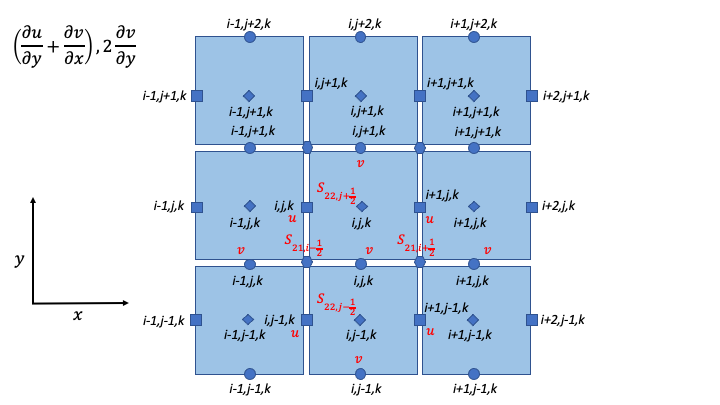
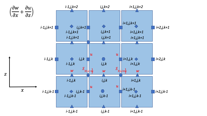
The schematic below (isomeric view) shows the definition of strain-rate components.
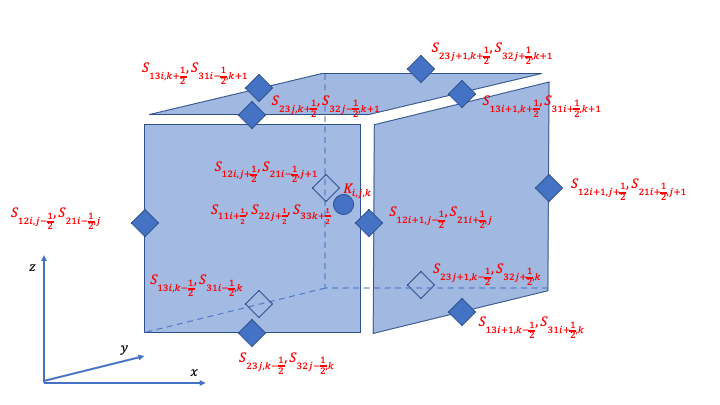
Strain-Rate Components for X-Momentum Equation
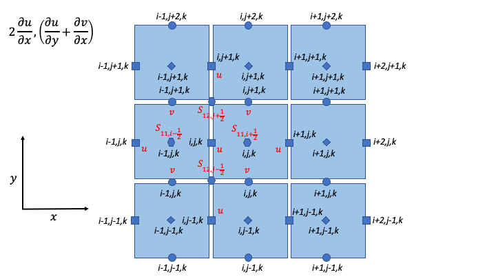
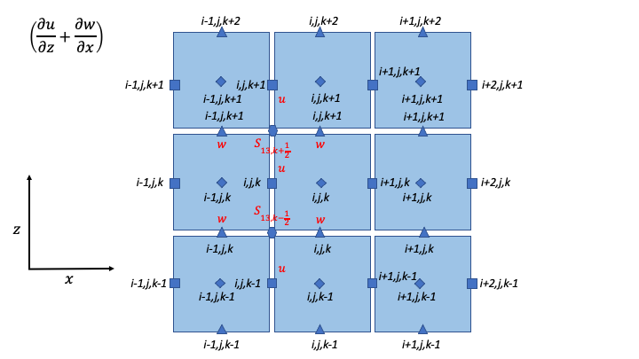
\[\begin{split}\begin{array}{ll}
S_{11,i + \frac{1}{2}} = & \frac{1}{\Delta x}\left( u_{i + 1,j,k} - u_{i,j,k} \right) \\
S_{11,i - \frac{1}{2}} = & \frac{1}{\Delta x}\left( u_{i,j,k} - u_{i - 1,j,k} \right) \\
S_{12,j + \frac{1}{2}} = & \frac{1}{2}\left\lbrack \frac{1}{\Delta y}\left( u_{i,j + 1,k} - u_{i,j,k} \right) + \frac{1}{\Delta x}\left( v_{i,j + 1,k} - v_{i - 1,j + 1,k} \right) \right\rbrack \\
S_{12,j - \frac{1}{2}} = & \frac{1}{2}\left\lbrack \frac{1}{\Delta y}\left( u_{i,j,k} - u_{i,j - 1,k} \right) + \frac{1}{\Delta x}\left( v_{i,j,k} - v_{i - 1,j,k} \right) \right\rbrack \\
S_{13,k + \frac{1}{2}} = & \frac{1}{2}\left\lbrack \frac{1}{\Delta z}\left( u_{i,j,k + 1} - u_{i,j,k} \right) + \frac{1}{\Delta x}\left( w_{i,j,k + 1} - w_{i - 1,j,k + 1} \right) \right\rbrack \\
S_{13,k - \frac{1}{2}} = & \frac{1}{2}\left\lbrack \frac{1}{\Delta z}\left( u_{i,j,k} - u_{i,j,k - 1} \right) + \frac{1}{\Delta x}\left( w_{i,j,k} - w_{i - 1,j,k} \right) \right\rbrack \\
\end{array}\end{split}\]
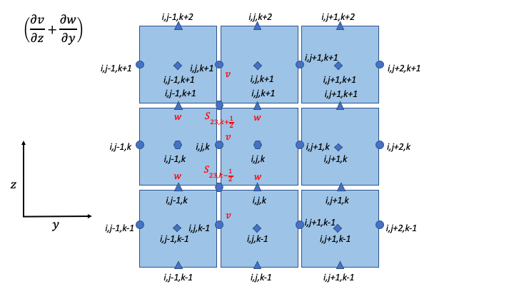
Strain-Rate Components for Y-Momentum Equation
\[\begin{split}\begin{array}{ll}
S_{21,i + \frac{1}{2}} = & \frac{1}{2}\left\lbrack \frac{1}{\Delta y}\left( u_{i + 1,j,k} - u_{i + 1,j - 1,k} \right) + \frac{1}{\Delta x}\left( v_{i + 1,j,k} - v_{i,j,k} \right) \right\rbrack \\
S_{21,i - \frac{1}{2}} = & \frac{1}{2}\left\lbrack \frac{1}{\Delta y}\left( u_{i,j,k} - u_{i,j - 1,k} \right) + \frac{1}{\Delta x}\left( v_{i,j,k} - v_{i - 1,j,k} \right) \right\rbrack \\
S_{22,j + \frac{1}{2}} = & \frac{1}{\Delta y}\left( v_{i,j + 1,k} - v_{i,j,k} \right) \\
S_{22,j - \frac{1}{2}} = & \frac{1}{\Delta y}\left( v_{i,j,k} - v_{i,j - 1,k} \right) \\
S_{23,k + \frac{1}{2}} = & \frac{1}{2}\left\lbrack \frac{1}{\Delta z}\left( v_{i,j,k + 1} - v_{i,j,k} \right) + \frac{1}{\Delta y}\left( w_{i,j,k + 1} - w_{i,j - 1,k + 1} \right) \right\rbrack \\
S_{23,k - \frac{1}{2}} = & \frac{1}{2}\left\lbrack \frac{1}{\Delta z}\left( v_{i,j,k} - v_{i,j,k - 1} \right) + \frac{1}{\Delta y}\left( w_{i,j,k} - w_{i,j - 1,k} \right) \right\rbrack \\
\end{array}\end{split}\]
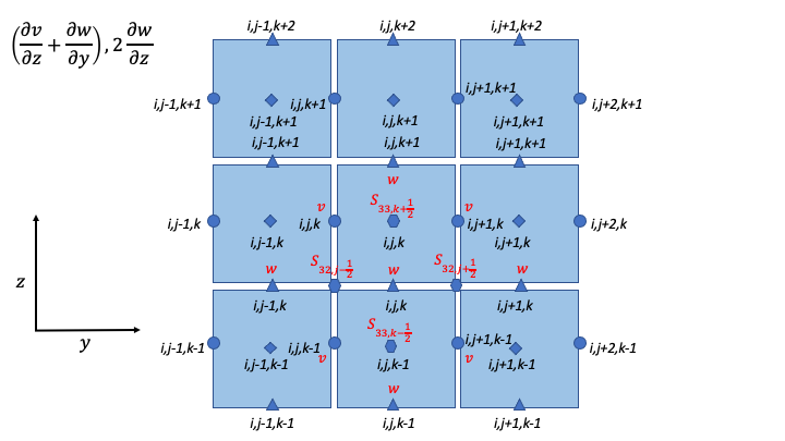
Strain-Rate Components for Z-Momentum Equation
\[\begin{split}\begin{array}{ll}
S_{31,i + \frac{1}{2}} = & \frac{1}{2}\left\lbrack \frac{1}{\Delta z}\left( u_{i + 1,j,k} - u_{i + 1,j,k - 1} \right) + \frac{1}{\Delta x}\left( w_{i + 1,j,k} - w_{i,j,k} \right) \right\rbrack \\
S_{31,i - \frac{1}{2}} = & \frac{1}{2}\left\lbrack \frac{1}{\Delta z}\left( u_{i,j,k} - u_{i,j,k - 1} \right) + \frac{1}{\Delta x}\left( w_{i,j,k} - w_{i - 1,j,k} \right) \right\rbrack \\
S_{32,j + \frac{1}{2}} = & \frac{1}{2}\left\lbrack \frac{1}{\Delta z}\left( v_{i,j + 1,k} - v_{i,j + 1,k - 1} \right) + \frac{1}{\Delta y}\left( w_{i,j + 1,k} - w_{i,j,k} \right) \right\rbrack \\
S_{32,j - \frac{1}{2}} = & \frac{1}{2}\left\lbrack \frac{1}{\Delta z}\left( v_{i,j,k} - v_{i,j,k - 1} \right) + \frac{1}{\Delta y}\left( w_{i,j,k} - w_{i,j - 1,k} \right) \right\rbrack \\
S_{33,k + \frac{1}{2}} = & \frac{1}{\Delta z}\left( w_{i,j,k + 1} - w_{i,j,k} \right) \\
S_{33,k - \frac{1}{2}} = & \frac{1}{\Delta z}\left( w_{i,j,k} - w_{i,j,k - 1} \right) \\
\end{array}\end{split}\]
Expansion-Rate Tensor
Expansion-Rate Components for X-Momentum Equation
\[\begin{split}\begin{array}{ll}
D_{11,i + \frac{1}{2}} = & \frac{1}{3}\left\lbrack \frac{1}{\Delta x}\left( u_{i + 1,j,k} - u_{i,j,k} \right) + \frac{1}{\Delta y}\left( v_{i,j + 1,k} - v_{i,j,k} \right) + \frac{1}{\Delta z}\left( w_{i,j,k + 1} - w_{i,j,k} \right) \right\rbrack \\
D_{11,i - \frac{1}{2}} = & \frac{1}{3}\left\lbrack \frac{1}{\Delta x}\left( u_{i,j,k} - u_{i-1,j,k} \right) + \frac{1}{\Delta y}\left( v_{i-1,j + 1,k} - v_{i-1,j,k} \right) + \frac{1}{\Delta z}\left( w_{i-1,j,k + 1} - w_{i-1,j,k} \right) \right\rbrack \\
D_{12,j + \frac{1}{2}} = & 0 \\
D_{12,j - \frac{1}{2}} = & 0 \\
D_{13,k + \frac{1}{2}} = & 0 \\
D_{13,k - \frac{1}{2}} = & 0 \\
\end{array}\end{split}\]
Expansion-Rate Components for Y-Momentum Equation
\[\begin{split}\begin{array}{ll}
D_{21,i + \frac{1}{2}} = & 0 \\
D_{21,i - \frac{1}{2}} = & 0 \\
D_{22,j + \frac{1}{2}} = & \frac{1}{3}\left\lbrack \frac{1}{\Delta x}\left( u_{i + 1,j,k} - u_{i,j,k} \right) + \frac{1}{\Delta y}\left( v_{i,j + 1,k} - v_{i,j,k} \right) + \frac{1}{\Delta z}\left( w_{i,j,k + 1} - w_{i,j,k} \right) \right\rbrack \\
D_{22,j - \frac{1}{2}} = & \frac{1}{3}\left\lbrack \frac{1}{\Delta x}\left( u_{i + 1,j-1,k} - u_{i,j-1,k} \right) + \frac{1}{\Delta y}\left( v_{i,j,k} - v_{i,j-1,k} \right) + \frac{1}{\Delta z}\left( w_{i,j-1,k + 1} - w_{i,j-1,k} \right) \right\rbrack \\
D_{23,k + \frac{1}{2}} = & 0 \\
D_{23,k - \frac{1}{2}} = & 0 \\
\end{array}\end{split}\]
Expansion-Rate Components for Z-Momentum Equation
\[\begin{split}\begin{array}{ll}
D_{21,i + \frac{1}{2}} = & 0 \\
D_{21,i - \frac{1}{2}} = & 0 \\
D_{22,j + \frac{1}{2}} = & 0 \\
D_{22,j - \frac{1}{2}} = & 0 \\
D_{23,k + \frac{1}{2}} = & \frac{1}{3}\left\lbrack \frac{1}{\Delta x}\left( u_{i + 1,j,k} - u_{i,j,k} \right) + \frac{1}{\Delta y}\left( v_{i,j + 1,k} - v_{i,j,k} \right) + \frac{1}{\Delta z}\left( w_{i,j,k + 1} - w_{i,j,k} \right) \right\rbrack \\
D_{23,k - \frac{1}{2}} = & \frac{1}{3}\left\lbrack \frac{1}{\Delta x}\left( u_{i + 1,j,k-1} - u_{i,j,k-1} \right) + \frac{1}{\Delta y}\left( v_{i,j + 1,k-1} - v_{i,j,k-1} \right) + \frac{1}{\Delta z}\left( w_{i,j,k} - w_{i,j,k-1} \right) \right\rbrack \\
\end{array}\end{split}\]
U Momentum viscous stress divergence
\[\begin{split}\begin{align}
\left( \rho u \right)_{i,j,k}^{n + 1} = \left( \rho u \right)_{i,j,k}^{n} - & \\
\Delta t & \left\{ \frac{1}{\Delta x}\ \left\lbrack \tau_{11,i + \frac{1}{2}} - \tau_{11,i - \frac{1}{2}} \right\rbrack \right.\ \\
& + \frac{1}{\Delta y}\ \left\lbrack \tau_{12,j + \frac{1}{2}} - \tau_{12,j - \frac{1}{2}} \right\rbrack \\
& + \left. \frac{1}{\Delta z}\ \left\lbrack \tau_{13,k + \frac{1}{2}} - \tau_{13,k - \frac{1}{2}} \right\rbrack \right\} \\
\end{align}\end{split}\]
Note that LES equation has a similar format for computing \(\tau_{11,i + \frac{1}{2}}\), \(\tau_{11,i - \frac{1}{2}}\),
\(\tau_{12,j + \frac{1}{2}}\), \(\tau_{12,j - \frac{1}{2}}\), \(\tau_{13,k + \frac{1}{2}}\),
and \(\tau_{13,k - \frac{1}{2}}\).
\[\begin{split}\begin{array}{ll}
\tau_{ij,m + \frac{1}{2}} = & -\mu_{eff} \ \left\lbrack S_{ij,m + \frac{1}{2}} - D_{ij,m + \frac{1}{2}} \right\rbrack \\
\tau_{ij,m - \frac{1}{2}} = & -\mu_{eff} \ \left\lbrack S_{ij,m - \frac{1}{2}} - D_{ij,m - \frac{1}{2}} \right\rbrack
\end{array}\end{split}\]
where \(m = i, j, k\).
\(\mu_{eff} = 2\mu\) if a constant molecular diffusion type is chosen (erf.molec_diff_type = "Constant").
Otherwise (erf.molec_diff_type = "None"), \(\mu_{eff} = 0\).
The nomenclature is similar for other two momentum equations. Note that \(\mu\) is constant in the current
implementation and its variation with temperature for low-Mach atmospheric flows has been ignored.
V Momentum viscous stress divergence
\[\begin{split}\begin{align}
\left( \rho v \right)_{i,j,k}^{n + 1} = \left( \rho v \right)_{i,j,k}^{n} - & \\
\Delta t & \left\{ \frac{1}{\Delta x} \left\lbrack \tau_{21,i + \frac{1}{2}} - \tau_{21,i - \frac{1}{2}} \right\rbrack \right. \\
& + \frac{1}{\Delta y} \left\lbrack \tau_{22,j + \frac{1}{2}} - \tau_{22,j - \frac{1}{2}} \right\rbrack \\
& + \left. \frac{1}{\Delta z} \left\lbrack \tau_{23,k + \frac{1}{2}} - \tau_{23,k - \frac{1}{2}} \right\rbrack \right\}
\end{align}\end{split}\]
Note that LES equation has a similar format for computing \(\tau_{21,i + \frac{1}{2}}\), \(\tau_{21,i - \frac{1}{2}}\),
\(\tau_{22,j + \frac{1}{2}}\), \(\tau_{22,j - \frac{1}{2}}\), \(\tau_{23,k + \frac{1}{2}}\),
and \(\tau_{23,k - \frac{1}{2}}\).
W Momentum viscous stress divergence
\[\begin{split}\begin{align}
\left( \rho w \right)_{i,j,k}^{n + 1} = \left( \rho w \right)_{i,j,k}^{n} - & \\
\Delta t & \left\{ \frac{1}{\Delta x} \left\lbrack \tau_{31,i + \frac{1}{2}} - \tau_{31,i - \frac{1}{2}} \right\rbrack \right. \\
& + \frac{1}{\Delta y} \left\lbrack \tau_{32,j + \frac{1}{2}} - \tau_{32,j - \frac{1}{2}} \right\rbrack \\
& + \left. \frac{1}{\Delta z} \left\lbrack \tau_{33,k + \frac{1}{2}} - \tau_{33,k - \frac{1}{2}} \right\rbrack \right\}
\end{align}\end{split}\]
Note that LES equation has a similar format for computing \(\tau_{31,i + \frac{1}{2}}\), \(\tau_{31,i - \frac{1}{2}}\),
\(\tau_{32,j + \frac{1}{2}}\), \(\tau_{32,j - \frac{1}{2}}\), \(\tau_{33,k + \frac{1}{2}}\),
and \(\tau_{33,k - \frac{1}{2}}\).
Potential Temperature Diffusion
\[\begin{split}\begin{matrix}
\left( \rho \theta \right)_{i,j,k}^{n + 1} & = & \left( \rho \theta \right)_{i,j,k}^{n} & + & \Delta t\rho_{i,j,k}\alpha_{T} & \left\{ \frac{1}{{\Delta x}^{2}}\ \left\lbrack \theta_{i + 1,j,k}^{n} - \ {2\theta}_{i,j,k}^{n} + \ \theta_{i - 1,j,k}^{n} \right\rbrack \right.\ \\
& & & & & + \frac{1}{{\Delta y}^{2}}\left\lbrack \theta_{i,j + 1,k}^{n} - \ 2\theta_{i,j,k}^{n} + \ \theta_{i,j - 1,k}^{n} \right\rbrack \\
& & & & & + \left. \frac{1}{{\Delta z}^{2}}\left\lbrack \theta_{i,j,k + 1}^{n} - \ {2\theta}_{i,j,k}^{n} + \ \theta_{i,j,k - 1}^{n} \right\rbrack \right\}
\end{matrix}\end{split}\]
Scalar Diffusion
\[\begin{split}\begin{matrix}
\left( \rho C \right)_{i,j,k}^{n + 1} & = & \left( \rho C \right)_{i,j,k}^{n} & + & \Delta t\rho_{i,j,k}\alpha_{C} & \left\{ \frac{1}{{\Delta x}^{2}}\ \left\lbrack C_{i + 1,j,k}^{n} - \ 2C_{i,j,k}^{n} + \ C_{i - 1,j,k}^{n} \right\rbrack \right.\ \\
& & & & & + \frac{1}{{\Delta y}^{2}}\left\lbrack C_{i,j + 1,k}^{n} - \ 2C_{i,j,k}^{n} + \ C_{i,j - 1,k}^{n} \right\rbrack \\
& & & & & + \left. \frac{1}{{\Delta z}^{2}}\left\lbrack C_{i,j,k + 1}^{n} - \ 2C_{i,j,k}^{n} + \ C_{i,j,k - 1}^{n} \right\rbrack \right\}
\end{matrix}\end{split}\]
Note: In WRF, the diffusion coefficients specified in the input file (\(K_h\) and \(K_v\) for horizontal and vertical diffusion) get divided by the Prandtl number for
the potential temperature and the scalars. For the momentum, they are used as it is. In ERF, the coefficients specified in the inputs (\(\alpha_T\) and \(\alpha_C\)) are used as it is, and no division by Prandtl number is done.
Scalar-diffusion field interface
For a cell-centered intensive scalar \(\chi\), ERF writes the signed
diffusive flux as
\[\mathbf{F}^D = -K \nabla \chi,\]
so its contribution to the conservative scalar equation is
\[\left.\frac{\partial(\rho\chi)}{\partial t}\right|_D
= -\nabla\cdot\mathbf{F}^D.\]
The effective transport coefficient \(K\) may contain molecular and
turbulent contributions. Coefficient selection is separate from scalar
identity: the native state adapter selects the thermal, TKE, passive-scalar,
or moisture coefficient category, while the numerical operator consumes an
explicit scalar component and coefficient policy. The scalar component,
density component, face-flux component, and output-tendency component are
independent. The non-embedded-boundary N, S, and T spatial operators therefore
do not require an arbitrary intensive scalar to be staged in ERF’s conserved
state layout.
The field-level entry points are BuildScalarDiffusionFluxes_N,
BuildScalarDiffusionFluxes_S, and BuildScalarDiffusionFluxes_T in
ERF_ScalarDiffusion.H. They construct the existing raw signed spatial
diffusion flux \(\mathbf{F}^D=-K\nabla\chi\). Separate
BuildScalarDiffusionMappedTransfers_N/S/T operations expose those
candidates in the same mapped face-transfer space used by reusable scalar
advection. The mapped transfer \(\widetilde F_d\) is an instantaneous
rate; it is not multiplied by \(dt\).
The authoritative discrete contract for a cell is
\[\frac{\partial U_i}{\partial t} =
-\frac{m_{x,i}m_{y,i}}{\mathrm{detJ}_i}
\left[
\frac{\widetilde F_{x,i+1/2}-\widetilde F_{x,i-1/2}}{\Delta\xi}+
\frac{\widetilde F_{y,j+1/2}-\widetilde F_{y,j-1/2}}{\Delta\eta}+
\frac{\widetilde F_{z,k+1/2}-\widetilde F_{z,k-1/2}}{\Delta\zeta}
\right], \qquad
H_i=\frac{\mathrm{detJ}_i}{m_{x,i}m_{y,i}}U_i.\]
Here detJ is the ERF cell metric supplied to the mapped divergence; for
terrain it stores \(h_\zeta\), while
\(\mathrm{detJ}/(m_xm_y)\) is the complete mapped cell-volume Jacobian
factor. The map factors \(m_x,m_y\) are the cell-centered mf_mx and
mf_my values. The mapped equation gives
\(\partial H_i/\partial t=-\sum_d\Delta_d\widetilde F_d/\Delta\xi_d\).
Geometry represented inside a face transfer must not be applied again. Each
shared face uses one supplied value for both neighboring cells, and callers
may modify a candidate before passing the accepted face arrays to
ApplyScalarMappedFluxDivergence. That operation reads only those arrays
and the mapped cell geometry. The face arrays and geometry convention match
ApplyScalarAdvectionFluxDivergence. Their RHS semantics differ:
ApplyScalarMappedFluxDivergence accumulates \(-\mathrm{div}\) into the
existing RHS and leaves cells with nonpositive detJ unchanged, while
ApplyScalarAdvectionFluxDivergence assigns its output and sets such cells
to zero.
The pointwise conversion helpers are GPU-callable so callers can materialize
transfers in fused or component-chunked kernels. The whole-array operations are
convenience wrappers around those helpers. For N geometry, the builder’s x/y
outputs already contain the horizontal map-factor ratios and are copied as the
x/y transfers; the vertical transfer is
\(\widetilde F_z=F_z^D/(m_xm_y)\). For S geometry, restore the vertical
Jacobian measure in the side faces and map the vertical flux as
\[\widetilde F_x=a_xF_x^S,\qquad
\widetilde F_y=a_yF_y^S,\qquad
\widetilde F_z=F_z^S/(m_xm_y).\]
Here ax and ay are the side-area/Jacobian measures, and detJ and
the computational \(\Delta\zeta\) supplied to the mapped divergence must
describe the same stretched coordinate. For a purely vertically stretched
mesh, ax = ay = detJ; this restores the native S-grid divergence, including
nonuniform physical cell widths.
For terrain-following coordinates, x/y transfers use the existing
TerrainDiffusionMappedTx and TerrainDiffusionMappedTy operations:
\[\widetilde F_x=F_x^T a_x/m_{u,y},\qquad
\widetilde F_y=F_y^T a_y/m_{v,x}.\]
At a k face, TerrainScalarDiffusionGzAtKFace remains the sole owner of
x/y-to-z interpolation, bottom/top extrapolation, terrain metrics, and cross
terms. It constructs
\[G_\zeta=F_z^T-m_xh_\xi\overline{F_x^T}
-m_yh_\eta\overline{F_y^T},\qquad
\widetilde F_z=G_\zeta/(m_xm_y).\]
TerrainScalarDiffusionMappedTransferAtKFace exposes the complete mapped
vertical transfer. Its explicit suppression argument sets the complete lower
transfer to zero when the resolved native boundary policy requires that
behavior; it does not merely zero raw \(F_z\) while retaining cross terms.
At an interior k face, its raw x/y inputs must be valid at kface and
kface-1. For whole-array materialization over cell box bx, when
bx.smallEnd(2) is above the domain bottom, raw x/y must include
bx.smallEnd(2)-1; when bx.bigEnd(2) is below the domain top, raw x/y
must include bx.bigEnd(2)+1. No outside-domain z layer is required at a
physical bottom or top face because the authoritative helper uses one-sided
extrapolation. Raw candidates from BuildScalarDiffusionFluxes_T already
meet this coverage requirement.
The whole-array T materializer launches its z mapping before its x/y mappings,
so corresponding raw and mapped directional arrays may alias in place,
including the same component. The launches use AMReX’s ordered execution
stream; cross-direction aliasing is not supported.
The native N/S/T source routines continue to consume their existing raw
representations and divergence paths. The external mapping API does not route
native ERF diffusion through the changed arithmetic association of mapped
transfers. Semi-implicit integration weights remain outside this mapping
layer: the conversion operates on whichever raw spatial candidate the caller
supplies, while ERF retains its existing scaling and diagnostic behavior.
This interface does not claim direct compatibility with YAFluxRegister or
another AMR flux register.
For semi-implicit vertical diffusion, ERF first constructs the full spatial
diffusion flux. The explicit/implicit split scales only the raw
\(F_z^D\) contribution. Unless erf.implicit_terrain_metric = true (see
Momentum stresses on terrain-fitted meshes), the terrain cross terms remain explicit, so the
explicit transformed numerator is
\[G_{\zeta,\mathrm{explicit}} =
(1-f_{\mathrm{implicit}})F_z^D
-m_xh_\xi\overline{F_x^D}-m_yh_\eta\overline{F_y^D}.\]
For momentum, each stage removes the implicit fraction of the correction stress
(\(\tau_{13}^i\), \(\tau_{23}^i\)) at the old state and solves the same flux back at
the new one. On the faces inside the domain and at coarse/fine boundaries, the two use the same
face coefficient and the same \(h_\zeta\) (the edge value by which the strain kernel divides
\(\partial u/\partial \zeta\)). With different values the split would change the operator
whatever the time step, wherever \(h_\zeta\) varies non-linearly between neighbouring
columns, as on curved terrain that decays with height. The split is not exact at a no-slip wall
(the correction stress uses a one-sided three-point \(\partial u/\partial z\), the solve the
two-point wall difference) and to first order in the density with erf.molec_diff_type = ConstantAlpha (the solve uses the predicted density).
With erf.implicit_terrain_metric = true the explicit numerator of the scalars becomes
\((1-f)F_z^D + f K_h M\, \partial\phi/\partial z - m_xh_\xi\overline{F_x^D}-m_yh_\eta\overline{F_y^D}\)
on the faces inside the domain.
Heat and moisture diagnostics continue to store the full raw vertical face
flux independently of this integration fraction. This is an implementation
interface and does not add a runtime option or change the configured diffusion
schemes. Embedded-boundary diffusion, implicit flux recovery, and AMR
diffusion reflux remain future work; the implicit tridiagonal solvers keep
their specialized implementations.
Momentum, Thermal, and Scalar Diffusion Contribution to LES
Strain Rate and Eddy Viscosity
The goal is to compute eddy viscosity at the cell centers and interpolated them to the edges. Refer again to the strain rate tensor schematic.
\[\begin{split}\begin{array}{ll}
S_{11} = & S_{11i + \frac{1}{2}} \\
S_{22} = & S_{22j + \frac{1}{2}} \\
S_{33} = & S_{33k + \frac{1}{2}}
\end{array}\end{split}\]
\[\begin{split}\begin{matrix}
S_{12} = & \frac{1}{4}\left\lbrack S_{12i,j - \frac{1}{2}} + S_{12i,j + \frac{1}{2}} + S_{12i + 1,j - \frac{1}{2}} + S_{12i + 1,j + \frac{1}{2}} \right\rbrack = \begin{smallmatrix} \text{Average of the 4 edges} \\ \text{surrounding the cell}\end{smallmatrix} \\
S_{21} = & \frac{1}{4}\left\lbrack S_{21i - \frac{1}{2},j} + S_{21i + \frac{1}{2},j} + S_{21i - \frac{1}{2},j + 1} + S_{21i + \frac{1}{2},j + 1} \right\rbrack = \begin{smallmatrix} \text{Average of the 4 edges} \\ \text{surrounding the cell}\end{smallmatrix} \\
S_{13} = & \frac{1}{4}\left\lbrack S_{13i,k - \frac{1}{2}} + S_{13i,k + \frac{1}{2}} + S_{13i + 1,k - \frac{1}{2}} + S_{13i + 1,k + \frac{1}{2}} \right\rbrack = \begin{smallmatrix} \text{Average of the 4 edges} \\ \text{surrounding the cell}\end{smallmatrix} \\
S_{31} = & \frac{1}{4}\left\lbrack S_{31i - \frac{1}{2},k} + S_{31i + \frac{1}{2},k} + S_{31i - \frac{1}{2},k + 1} + S_{31i + \frac{1}{2},k + 1} \right\rbrack = \begin{smallmatrix} \text{Average of the 4 edges} \\ \text{surrounding the cell}\end{smallmatrix} \\
S_{23} = & \frac{1}{4}\left\lbrack S_{23j,k - \frac{1}{2}} + S_{23j,k + \frac{1}{2}} + S_{23j + 1,k - \frac{1}{2}} + S_{23j + 1,k + \frac{1}{2}} \right\rbrack = \begin{smallmatrix} \text{Average of the 4 edges} \\ \text{surrounding the cell}\end{smallmatrix} \\
S_{32} = & \frac{1}{4}\left\lbrack S_{32j - \frac{1}{2},k} + S_{32j + \frac{1}{2},k} + S_{32j - \frac{1}{2},k + 1} + S_{32j + \frac{1}{2},k + 1} \right\rbrack = \begin{smallmatrix} \text{Average of the 4 edges} \\ \text{surrounding the cell}\end{smallmatrix}
\end{matrix}\end{split}\]
Note that:
\[\begin{split}\begin{array}{ll}
S_{12} = & S_{21} \\
S_{13} = & S_{31} \\
S_{23} = & S_{32}
\end{array}\end{split}\]
\(K_{i,j,k} = {2\left( C_{S}\ \Delta \right)^{2}\left( {2S}_{mn}S_{mn} \right)}^{\frac{1}{2}} \ \rho_{i,j,k}\),
where
\[\begin{split}S_{mn}S_{mn} = S_{11}^{2} + S_{22}^{2} + S_{33}^{2} + S_{12}^{2} + S_{13}^{2} + S_{23}^{2} + S_{21}^{2} + S_{31}^{2} + S_{32}^{2} \\\end{split}\]
Owing to symmetry we need to compute 6 of the 9 tensor components.
\(K_{i,j,k} = 2 \ {\mu_{t}}_{i, j, k}\) is the modeled turbulent viscosity and can be considered analogous to
\(2\mu_{i, j, k}\).
\(\mu_{eff} = 2\mu + K = 2\mu + 2\mu_{t}\) if a constant molecular diffusion type is chosen (erf.molec_diff_type = "Constant").
Otherwise (erf.molec_diff_type = "None"), \(\mu_{eff} = K = 2\mu_{t}\).
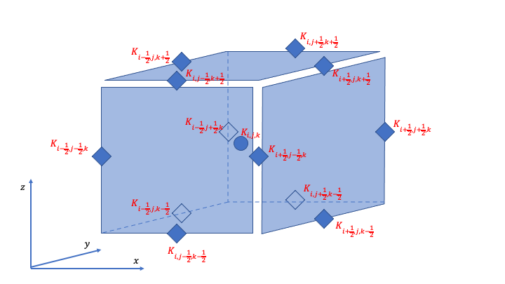
The interpolated values of eddy-viscosity at the edges are the average
of the values at the centers of the 4 cells the edge is part of.
\[\begin{split}\begin{array}{c}
K_{i + \frac{1}{2},j - \frac{1}{2},k} = \frac{1}{4}\left\lbrack K_{i,j - 1,k} + K_{i,j,k} + K_{i + 1,j - 1,k} + K_{i + 1,j,k} \right\rbrack \\
K_{i + \frac{1}{2},j + \frac{1}{2},k} = \frac{1}{4}\left\lbrack K_{i,j,k} + K_{i,j + 1,k} + K_{i + 1,j,k} + K_{i + 1,j + 1,k} \right\rbrack \\
K_{i + \frac{1}{2},j,k - \frac{1}{2}} = \frac{1}{4}\left\lbrack K_{i,j,k} + K_{i,j,k - 1} + K_{i + 1,j,k} + K_{i + 1,j,k - 1} \right\rbrack \\
K_{i + \frac{1}{2},j,k + \frac{1}{2}} = \frac{1}{4}\left\lbrack K_{i,j,k + 1} + K_{i,j,k} + K_{i + 1,j,k + 1} + K_{i + 1,j,k} \right\rbrack \\
K_{i,j + \frac{1}{2},k - \frac{1}{2}} = \frac{1}{4}\left\lbrack K_{i,j,k} + K_{i,j,k - 1} + K_{i,j + 1,k} + K_{i,j + 1,k - 1} \right\rbrack \\
K_{i,j + \frac{1}{2},k + \frac{1}{2}} = \frac{1}{4}\left\lbrack K_{i,j,k} + K_{i,j,k + 1} + K_{i,j + 1,k} + K_{i,j + 1,k + 1} \right\rbrack
\end{array}\end{split}\]
U Momentum - subfilter stress divergence
\[\begin{split}\begin{align}
\left( \rho u \right)_{i,j,k}^{n + 1} = \left( \rho u \right)_{i,j,k}^{n} - & \\
\Delta t & \left\{ \frac{1}{\Delta x}\ \left\lbrack \tau_{11,i + \frac{1}{2}} - \tau_{11,i - \frac{1}{2}} \right\rbrack \right.\ \\
& + \frac{1}{\Delta y}\ \left\lbrack \tau_{12,j + \frac{1}{2}} - \tau_{12,j - \frac{1}{2}} \right\rbrack \\
& + \left. \frac{1}{\Delta z}\ \left\lbrack \tau_{13,k + \frac{1}{2}} - \tau_{13,k - \frac{1}{2}} \right\rbrack \right\} \\
\end{align}\end{split}\]
\[\begin{split}\begin{array}{l}
\tau_{11,i + \frac{1}{2}} = -K_{i,j,k} \ S_{11,i + \frac{1}{2}} \\
\tau_{11,i - \frac{1}{2}} = -K_{i - 1,j,k} \ S_{11,i - \frac{1}{2}} \\
\tau_{12,j + \frac{1}{2}} = -K_{i - \frac{1}{2},j + \frac{1}{2},k} \ S_{12,j + \frac{1}{2}} \\
\tau_{12,j - \frac{1}{2}} = -K_{i - \frac{1}{2},j - \frac{1}{2},k} \ S_{12,j - \frac{1}{2}} \\
\tau_{13,k + \frac{1}{2}} = -K_{i - \frac{1}{2},j,k + \frac{1}{2}} \ S_{13,k + \frac{1}{2}} \\
\tau_{13,k - \frac{1}{2}} = -K_{i - \frac{1}{2},j,k - \frac{1}{2}} \ S_{13,k - \frac{1}{2}}
\end{array}\end{split}\]
V Momentum - subfilter stress divergence
\[\begin{split}\begin{align}
\left( \rho v \right)_{i,j,k}^{n + 1} = \left( \rho v \right)_{i,j,k}^{n} - & \\
\Delta t & \left\{ \frac{1}{\Delta x} \left\lbrack \tau_{21,i + \frac{1}{2}} - \tau_{21,i - \frac{1}{2}} \right\rbrack \right. \\
& + \frac{1}{\Delta y} \left\lbrack \tau_{22,j + \frac{1}{2}} - \tau_{22,j - \frac{1}{2}} \right\rbrack \\
& + \left. \frac{1}{\Delta z} \left\lbrack \tau_{23,k + \frac{1}{2}} - \tau_{23,k - \frac{1}{2}} \right\rbrack \right\}
\end{align}\end{split}\]
\[\begin{split}\begin{array}{ll}
\tau_{21,i + \frac{1}{2}} = -K_{i + \frac{1}{2},j - \frac{1}{2},k} \ S_{21,i + \frac{1}{2}} \\
\tau_{21,i - \frac{1}{2}} = -K_{i - \frac{1}{2},j - \frac{1}{2},k} \ S_{21,i - \frac{1}{2}} \\
\tau_{22,j + \frac{1}{2}} = -K_{i,j,k} \ S_{22,j + \frac{1}{2}} \\
\tau_{22,j - \frac{1}{2}} = -K_{i,j - 1,k} \ S_{22,j - \frac{1}{2}} \\
\tau_{23,k + \frac{1}{2}} = -K_{i,j - \frac{1}{2},k + \frac{1}{2}} \ S_{23,k + \frac{1}{2}} \\
\tau_{23,k - \frac{1}{2}} = -K_{i,j - \frac{1}{2}k - \frac{1}{2}} \ S_{23,k - \frac{1}{2}}
\end{array}\end{split}\]
W Momentum - subfilter stress divergence
\[\begin{split}\begin{align}
\left( \rho w \right)_{i,j,k}^{n + 1} = \left( \rho w \right)_{i,j,k}^{n} - & \\
\Delta t & \left\{ \frac{1}{\Delta x} \left\lbrack \tau_{31,i + \frac{1}{2}} - \tau_{31,i - \frac{1}{2}} \right\rbrack \right. \\
& + \frac{1}{\Delta y} \left\lbrack \tau_{32,j + \frac{1}{2}} - \tau_{32,j - \frac{1}{2}} \right\rbrack \\
& + \left. \frac{1}{\Delta z} \left\lbrack \tau_{33,k + \frac{1}{2}} - \tau_{33,k - \frac{1}{2}} \right\rbrack \right\}
\end{align}\end{split}\]
\[\begin{split}\begin{array}{ll}
\tau_{31,i + \frac{1}{2}} = -K_{i + \frac{1}{2},j,k - \frac{1}{2}} \ S_{31,i + \frac{1}{2}} \\
\tau_{31,i - \frac{1}{2}} = -K_{i - \frac{1}{2},j,k - \frac{1}{2}} \ S_{31,i - \frac{1}{2}} \\
\tau_{32,j + \frac{1}{2}} = -K_{i,j + \frac{1}{2},k - \frac{1}{2}} \ S_{32,j + \frac{1}{2}} \\
\tau_{32,j - \frac{1}{2}} = -K_{i,j - \frac{1}{2},k - \frac{1}{2}} \ S_{32,j - \frac{1}{2}} \\
\tau_{33,k + \frac{1}{2}} = -K_{i,j,k} \ S_{33,k + \frac{1}{2}} \\
\tau_{33,k - \frac{1}{2}} = -K_{i,j, k - 1} \ S_{33,k - \frac{1}{2}}
\end{array}\end{split}\]
Momentum stresses on terrain-fitted meshes
On a terrain-fitted mesh (ComputeStrain_T and ComputeStressVarVisc_T), the strains are
taken along the coordinate surfaces with the chain rule. For example,
\[S_{11} = m_x \left( \frac{\partial u}{\partial \xi} - h_\xi \frac{\partial u}{\partial z} \right),\]
where \(h_\xi = \partial z / \partial \xi\) and \(h_\eta = \partial z / \partial \eta\) are the
terrain slopes. The cell-centred \(\partial u / \partial z\) in \(S_{11}\) is the average
over the four \(x\)-\(z\) edges of the cell, so it uses the cell’s own faces
\(i\) and \(i+1\); \(\partial v / \partial z\) in \(S_{22}\) likewise uses the faces
\(j\) and \(j+1\).
The flux through a \(\zeta\) face is the stress projected onto the face normal. With
\(\nu_v\) and \(\nu_h\) the vertical and horizontal eddy viscosities as the code stores
them (EddyDiff::Mom_v and EddyDiff::Mom_h, density-weighted, each with the molecular
viscosity added) and the stress \(\tau_{ij} = -2\nu S_{ij}\),
\[\tau_{\zeta,1} = -2\left[ \nu_v\, S_{13}
- \left( h_\xi m_x \overline{\nu_h S_{11}} + h_\eta m_y \overline{\nu_h S_{12}} \right) \right],
\qquad
\tau_{\zeta,2} = -2\left[ \nu_v\, S_{23}
- \left( h_\xi m_x \overline{\nu_h S_{21}} + h_\eta m_y \overline{\nu_h S_{22}} \right) \right].\]
\(\nu_v\) is averaged to the edge from the four cells around it. The overbars average the
horizontal stresses where they are formed – \(\nu_h S_{11}\) and \(\nu_h S_{22}\) at the four
cells, \(\nu_h S_{12}\) at the four \(x\)-\(y\) edges, with \(\nu_h\) averaged to those
edges as for \(\tau_{12}\) – just as the scalars average their horizontal fluxes in
\(G_\zeta\) above. \(S_{11}\), \(S_{12}\) and \(S_{22}\) are horizontal strains, so
their projections take \(\nu_h\). In ERF’s symmetric stress tensor \(S_{31}\) and
\(S_{32}\) are vertical stresses, so the \(w\) equation’s \(\zeta\) flux projects them
with \(\nu_v\) (WRF uses the horizontal viscosity for the horizontal flux of \(w\)).
For the strain part of the stress (without the \(-\tfrac{1}{3}\) expansion-rate term) on a
uniform slope, with uniform vertical spacing and constant map factors, and away from the extrapolated
bottom and top planes, this makes the discrete operator dissipative for any
\(\nu_h, \nu_v \ge 0\): summation by parts gives a kinetic-energy rate of
\(-2\left[ \sum \nu_h (S_{11}^2 + S_{22}^2 + 2S_{12}^2) + \sum \nu_v (\ldots) \right] \le 0\),
because averaging \(\nu_h S_{11}\) to the edges is the transpose of the four-edge average in its
\(\partial u / \partial z\). Multiplying an edge-averaged \(\nu_h\) by the averaged strain
instead is not: where \(\nu_h\) changes from cell to cell, a grid-scale oblique wave can gain
energy (Tests/Unit/Diffusion/ERF_GTestTerrainStress.cpp has such a case). The expansion-rate
term is outside this argument: with \(\nu_h \ne \nu_v\) the deviatoric stresses are not
dissipative even in the continuum.
Where the slope varies, the transpose relation is no longer exact, and the operator need not
dissipate energy. An eigenvalue analysis of the assembled momentum operator, without the
expansion-rate term, on steep curved terrain (largest \(h \Delta x/\Delta z\) about 25, a sine of
four or eight cells’ wavelength, in 2-D and 3-D) found:
with \(\nu_h/\nu_v \gtrsim 100\), directions that gain energy; the largest transient growth
in the cases analysed was 1.9 in amplitude;
in every case, every eigenvalue with a negative real part, so no mode of the semi-discrete
operator (without the expansion-rate term) grows;
with the projected terms on \(\nu_v\), as before #4214, the same terrain had growing modes.
TerrainStress.CurvedSlopeOperatorHasNoGrowingMode checks this on such terrain.
Before erf-model/ERF#4214 the projected terms took \(\nu_v\). For \(u\) alone the rate was
then the quadratic form
\(2\nu_h a^2 - 2(\nu_h+\nu_v) h_\xi a b + \nu_v (1 + 2h_\xi^2) b^2\) in
\(a = \partial u/\partial \xi\) and \(b = \partial u/\partial z\). That form is indefinite when
\((\nu_h+\nu_v)^2 h_\xi^2 > 2\nu_h\nu_v(1+2h_\xi^2)\), which for \(\nu_h \gg \nu_v\) and
\(h_\xi^2 \ll 1\) is \(\nu_h h_\xi^2 > 2 \nu_v\), and which holds for any slope when
\(\nu_h = 0\). Oblique short waves were then amplified at a rate that does not depend on the
time step.
Runs on a flat terrain-fitted mesh are unchanged (bit for bit in the regression suite). On a sloped
mesh the answers of runs
with \(\nu_h \ne \nu_v\) change most:
erf.les_type = Smagorinsky2D;
Smagorinsky or Deardorff with erf.mix_isotropic = false;
any LES closure combined with a PBL scheme, which sets \(\nu_v\) only;
a PBL scheme without an LES closure. No PBL scheme sets \(\nu_h\), so it is the molecular
viscosity alone (usually zero) and the projected horizontal stresses drop out, as in WRF with a
PBL scheme, where the PBL mixes only in the vertical.
Runs with \(\nu_h = \nu_v\) (isotropic Smagorinsky or Deardorff, the k-equation closures)
change less, where the viscosity varies between neighbouring cells, because the average of
\(\nu S\) differs from the product of the averages. Runs with only a molecular viscosity
(ComputeStressConsVisc_T) change through the \(\partial u / \partial z\) correction, and
all three, with the implicit vertical solve on (the default), also through the exact implicit split
described below, where \(h_\zeta\) varies non-linearly between columns. The
\(\partial u / \partial z\) correction (also erf-model/ERF#4214) changes every run on a sloped
mesh where \(\partial u / \partial z\) varies along \(x\) (or \(\partial v / \partial z\)
along \(y\)), by what was a first-order error of about
\(\Delta x\, h_\xi\, \partial^2 u/\partial x \partial z\) in \(S_{11}\), which grows with the
slope. Through the
strain rate it also changes the Smagorinsky eddy viscosities and the shear production of the TKE
closures.
The projected horizontal stresses contain \(h_\xi\,\partial u/\partial z\) and
\(h_\eta\,\partial u/\partial z\), so the \(\zeta\) flux of \(u\) holds a vertical
diffusion \(-K_h M_u\, \partial u / \partial z\) with \(M_u = \tfrac{4}{3}(h_\xi m_x)^2 + (h_\eta m_y)^2\)
(\(M_v = (h_\xi m_x)^2 + \tfrac{4}{3}(h_\eta m_y)^2\) for \(v\), and
\(M = (h_\xi m_x)^2 + (h_\eta m_y)^2\) for the scalars). The factor \(\tfrac{4}{3}\)
comes from the deviatoric \(S_{11} - \tfrac{1}{3}\nabla\cdot\mathbf{u}\): \(S_{11}\) carries
\(-h_\xi m_x\, \partial u/\partial z\), and the expansion rate carries the same term, so the
deviator carries \(\tfrac{2}{3}\) of it. The vertical implicit solve treats
only \(K_v\), so this term is explicit and limits the time step on steep slopes when
\(K_h M \gg K_v\). With erf.implicit_terrain_metric = true its compact form
\(K_h M (\phi_k - \phi_{k-1})/\Delta z\) is added to the coefficients of the implicit solve on
every face inside the domain and subtracted from the explicit flux on the same faces
(ERF_TerrainImplicitMetric.H); the explicit operator keeps the averaged form, so only the
difference between the two stays explicit. That difference is small for smooth fields on a uniform
slope, but not where the slope or the viscosity changes from cell to cell, and not at the grid scale:
the averaged form does not see a \(2\Delta z\) wave, so there the explicit part is the whole
compact term with the opposite sign, cancelled within the stage by the implicit solve. The option
therefore needs the implicit solve in every Runge-Kutta stage (erf.vert_implicit_fac positive in
all three); in a stage without it the whole averaged metric term is explicit.
The WRF-based alternative, erf.smag2d_slope_limiter (Smagorinsky2D limits on terrain-fitted meshes),
reduces \(K_h\) on slopes instead of solving the term implicitly. With the option on, the
diffusive time-step check (erf.diffusive_dt_check) counts the \(K_h\) metric term with the
explicit fraction of the vertical diffusion.
Energy Conservation- Subgrid heat flux
\[\begin{split}\begin{align}
\left( \rho \theta \right)_{i,j,k}^{n + 1} = \left( \rho \theta \right)_{i,j,k}^{n} - & \\
& \Delta t \left\{ \frac{1}{\Delta x^2} \left\lbrack
K_{i+\frac{1}{2},j,k} (\theta_{i+1,j,k}^{n} - \theta_{i ,j,k}^{n}) -
K_{i-\frac{1}{2},j,k} (\theta_{i ,j,k}^{n} - \theta_{i-1,j,k}^{n}) \right\rbrack \right. \\
& + \frac{1}{\Delta y^2} \left\lbrack
K_{i,j+\frac{1}{2},k} (\theta_{i,j+1,k}^{n} - \theta_{i,j ,k}^{n}) -
K_{i,j-\frac{1}{2},k} (\theta_{i,j ,k}^{n} - \theta_{i,j-1,k}^{n}) \right\rbrack \\
& \left. + \frac{1}{\Delta z^2} \left\lbrack
K_{i,j,k-\frac{1}{2}} (\theta_{i,j,k+1}^{n} - \theta_{i,j,k }^{n})
K_{i,j,k-\frac{1}{2}} (\theta_{i,j,k }^{n} - \theta_{i,j,k-1}^{n}) \right\rbrack \right\}
\end{align}\end{split}\]
Analogous formulae apply for the subgrid scalar flux.
Prognostic Equation for Subgrid Kinetic Energy
\[\begin{split}\begin{align}
\left( \rho e \right)_{i,j,k}^{n + 1} = \left( \rho e \right)_{i,j,k}^{n} - & \\
\Delta t & \left\{ \frac{1}{\Delta x}\left\lbrack \left( \rho u \right)_{i+1,j,k}^{n}e_{i+\frac{1}{2},j,k}^{n}
- \left( \rho u \right)_{i ,j,k}^{n}e_{i-\frac{1}{2},j,k}^{n} \right\rbrack \right. \\
& + \frac{1}{\Delta y}\left\lbrack \left( \rho v \right)_{i,j+1,k}^{n}e_{i,j+\frac{1}{2},k}^{n}
- \left( \rho v \right)_{i,j ,k}^{n}e_{i,j-\frac{1}{2},k}^{n} \right\rbrack \\
& + \frac{1}{\Delta z}\left\lbrack \left( \rho w \right)_{i,j,k+1}^{n}e_{i,j,k+\frac{1}{2}}^{n}
- \left( \rho w \right)_{i,j,k }^{n}e_{i,j,k-\frac{1}{2}}^{n} \right\rbrack \\
& + \left. \frac{g}{\theta_{i,j,k}} \frac{1}{2} \left\lbrack (\rho K_H \frac{\partial\theta}{\partial z})_{i,j,k-\frac{1}{2}} + (\rho K_H \frac{\partial\theta}{\partial z})_{i,j,k+\frac{1}{2}} \right\rbrack
- \tau_{mn}\frac{\partial u_{m}}{\partial x_{n}}
+ (\nabla \cdot (K \nabla e))_{i,j,k}
- \rho_{i,j,k} C_{\epsilon} \frac{\left( e_{i,j,k} \right)^{\frac{3}{2}}}{\mathcal{l}} \right\}
\end{align}\end{split}\]
where
\[\begin{split}\begin{array}{l}
C_{\epsilon} = 0.19 + 0.51\frac{\mathcal{l}}{\Delta s} \\
K_{H} = \left( 1 + 2\frac{\mathcal{l}}{\Delta s} \right)K_{M} \\
K_{M} = 0.1 \mathcal{l} e^{\frac{1}{2}}
\end{array}\end{split}\]
For convective or neutral cases, \(\theta^{n}_{i,j,k+1}-\theta^{n}_{i,j,k-1} < 0\), \(\mathcal{l} = \Delta s = \sqrt[3]{\Delta x \Delta y \Delta z}\)
For stable cases, \(\theta^{n}_{i,j,k+1}-\theta^{n}_{i,j,k-1} > 0\),
\[\begin{split}\begin{align}
\mathcal{l} & = 0.76\ e^{\frac{1}{2}}\left( \frac{g}{\theta}\frac{\partial\theta}{\partial z} \right) \\
& = 0.76e_{i,j,k}^{\frac{1}{2}}\left\lbrack \frac{g}{\theta_{i,j,k}}\frac{1}{2\Delta z}\left( \theta_{i,j,k + 1}^{n} - \theta_{i,j,k - 1}^{n} \right) \right\rbrack
\end{align}\end{split}\]
The second to last term on the right hand side takes the form
\[\begin{split}\begin{align}
& \frac{1}{\Delta x^2} \left\lbrack
K_{i+\frac{1}{2},j,k} (e_{i+1,j,k}^{n} - e_{i ,j,k}^{n}) -
K_{i-\frac{1}{2},j,k} (e_{i ,j,k}^{n} - e_{i-1,j,k}^{n}) \right\rbrack + \\
& \frac{1}{\Delta y^2} \left\lbrack
K_{i,j+\frac{1}{2},k} (e_{i,j+1,k}^{n} - e_{i,j ,k}^{n}) -
K_{i,j-\frac{1}{2},k} (e_{i,j ,k}^{n} - e_{i,j-1,k}^{n}) \right\rbrack + \\
& \frac{1}{\Delta z^2} \left\lbrack
K_{i,j,k-\frac{1}{2}} (e_{i,j,k+1}^{n} - e_{i,j,k }^{n}) -
K_{i,j,k-\frac{1}{2}} (e_{i,j,k }^{n} - e_{i,j,k-1}^{n}) \right\rbrack
\end{align}\end{split}\]
Finally,
\[\begin{split}\begin{align}
\tau_{mn}\frac{\partial u_{m}}{\partial x_{n}} & = K S_{mn}\frac{\partial u_{m}}{\partial x_{n}} \\
& = K S_{mn}S_{mn} \\
& = K (S_{11}^{2} + S_{22}^{2} + S_{33}^{2} + S_{12}^{2} + S_{13}^{2} + S_{23}^{2} + S_{21}^{2} + S_{31}^{2} + S_{32}^{2})
\end{align}\end{split}\]
Contributions from different directions