Domain Boundary Condition Types
Lateral boundary conditions in ERF can be specified for idealized simulations as periodic, inflow, outflow, or open. More realistic conditions include the use of time-varying values read in from external files, such as the wrfbdy files generated by the WRF Preprocessing System (WPS). ERF also has the option to run precursor simulations, save planes of data at specified times, and later read boundary data from those files analogously to how data from the wrfbdy are used.
The bottom surface boundary condition can be specified as a simple wall or by using Monin-Obukhov similarity theory (MOST). When utilizing MOST, the surface roughness, \(z_0\), may be specified as a constant, read from a file, or dynamically computed from the Charnock or shallow water formulation. Time-varying sea surface temperatures may also be employed in conjunction with MOST.
Ideal Domain BCs
There are two primary types of physical/domain boundary conditions: those which rely only on the data in the valid regions, and those which rely on externally specified values.
ERF allows users to specify types of boundary condition with keywords in the inputs file.
The information for each face is preceded by
xlo, xhi, ylo, yhi, zlo, or zhi.
Currently available type of boundary conditions are
inflow, outflow, inflow_outflow, slipwall, noslipwall, symmetry or surface_layer.
(Spelling of the type matters; capitalization does not.)
For example, setting
xlo.type = "inflow"
xhi.type = "outflow"
zlo.type = "slipwall"
zhi.type = "slipwall"

geometry.is_periodic = 0 1 0
would define a problem with inflow in the low-\(x\) direction,
outflow in the high-\(x\) direction, periodic in the \(y\)-direction,
and slip wall on the low and high \(y\)-faces, and
Note that no keyword is needed for a periodic boundary, here only the
specification in geometry.is_periodic is needed.
Each of these types of physical boundary condition has a mapping to a mathematical boundary condition for each type; this is summarized in the table below.
ERF provides the ability to specify a variety of boundary conditions (BCs) in the inputs file.
We use the following options preceded by xlo, xhi, ylo, yhi, zlo, and zhi:
Type |
Normal vel |
Tangential vel |
Density |
Theta |
Scalar |
|---|---|---|---|---|---|
inflow |
ext_dir |
ext_dir |
ext_dir |
ext_dir |
ext_dir |
outflow |
foextrap |
foextrap |
foextrap |
foextrap |
foextrap |
inflowoutflow |
ext_dir if inflowing; otherwise foextrap |
ext_dir if inflowing; otherwise foextrap |
ext_dir if inflowing; otherwise foextrap |
ext_dir if inflowing; otherwise foextrap |
ext_dir if inflowing; otherwise foextrap |
slipwall |
ext_dir |
foextrap |
foextrap |
ext_dir/foextrap/neumann |
foextrap |
noslipwall |
ext_dir |
ext_dir |
foextrap |
ext_dir/foextrap/neumann |
foextrap |
symmetry |
reflect_odd |
reflect_even |
reflect_even |
reflect_even |
reflect_even |
surface_layer |
ext_dir |
hoextrap |
hoextrap |
hoextrap |
hoextrap |
Here ext_dir, foextrap, and reflect_even refer to AMReX keywords. The ext_dir type
refers to an “external Dirichlet” boundary, which means the values must be specified by the user.
The foextrap type refers to “first order extrapolation” which sets all the ghost values to the
same value in the last valid cell/face. By contrast, hoextrap, or “higher order extrapolation”,
does a linear extrapolation from the two nearest valid values. The neumann condition
is an ERF-specific boundary type that allows a user to specify a variable gradient. Currently, the
neumann BC is only supported for theta to allow for weak capping inversion
(\(\partial \theta / \partial z\)) at the top domain. The surface_layer condition is an ERF-specific
boundary type that employs the above set of boundary conditions but also directly specifies the
subgrid scale diffusive fluxes; see Surface Layer Boundaries for more information.
As an example,
xlo.type                =   inflow
xlo.velocity            =   1. 0.9  0.
xlo.density             =   1.
xlo.theta               =   300.
xlo.scalar              =   2.
sets the boundary condition type at the low x face to be an inflow with xlo.type = “inflow”.
xlo.velocity = 1. 0. 0. sets all three componentns the inflow velocity, xlo.density = 1. sets the inflow density, xlo.theta = 300. sets the inflow potential temperature, xlo.scalar = 2. sets the inflow value of the advected scalar
Non-reflecting inflow
By default, the inflow boundary prescribes Dirichlet values for all variables
including \(\rho\theta\), which implicitly fixes the pressure in the ghost cells.
This causes upstream-propagating acoustic waves to reflect off the boundary,
which can destabilize simulations with terrain or other pressure perturbation sources.
Setting nonreflecting = true on an inflow face switches the \(\rho\theta\)
boundary condition from ext_dir to foextrap (zero-gradient extrapolation from
the interior) while keeping velocity and density prescribed. This allows the outgoing
acoustic characteristic (pressure) to exit the domain.
xlo.type            = “Inflow”
xlo.velocity        = 10. 0. 0.
xlo.density         = 1.16
xlo.theta           = 300.
xlo.nonreflecting   = true
Additionally, one may use an input file to specify the Dirichlet velocities as a function of the
vertical coordinate z. The input file is expected to contain either {z u v w} or
{z u v w theta} and is currently only available for the xlo face. For a file
named inflow_file that contains the variables {z u v w}, one would use
the inputs below; note, that if the inflow file contains {z u v w theta} then the
below example should be modified to not include xlo.theta = <val>.
If theta is provided, it is by default the primitive variable, not the conserved quantity
rho*theta. To specify rho*theta instead, xlo.read_prim_theta = false should be set.
xlo.type                =   "inflow"
xlo.dirichlet_file      =   "inflow_file"
xlo.density             =   1.
xlo.theta               =   300.
xlo.scalar              =   2.
The slipwall and noslipwall types have options for adiabatic vs Dirichlet boundary conditions.
If a value for theta is given for a face with type slipwall or noslipwall then the boundary
condition for theta is assumed to be “ext_dir”, i.e. theta is specified on the boundary.
If no value is specified then the wall is assumed to be adiabiatc, i.e. there is no temperature
flux at the boundary. This is enforced with the “foextrap” designation.
For example
zlo.type  = "NoSlipWall"
zhi.type  = "NoSlipWall"

zlo.theta = 301.0
would designate theta = 301 at the bottom (zlo) boundary, while
the top boundary condition would default to a zero gradient (adiabatic)
since no value is specified for zhi.theta or zhi.theta_grad.
By contrast, thermal inversion may be imposed at the top boundary
by providing a specified gradient for theta
zlo.type  = "NoSlipWall"
zhi.type  = "NoSlipWall"

zlo.theta = 301.0
zhi.theta_grad = 1.0
We note that noslipwall allows for non-zero tangential velocities to be specified, as in the
Couette regression test example, in which we specify
geometry.is_periodic = 1 1 0

zlo.type = "NoSlipWall"
zhi.type = "NoSlipWall"

zlo.velocity    = 0.0 0.0 0.0
zhi.velocity    = 2.0 0.0 0.0
We also note that in the case of a slipwall boundary condition in a simulation with non-zero
viscosity specified, the “foextrap” boundary condition enforces zero strain at the wall.
It is important to note that external Dirichlet boundary data should be specified as the value on the face of the cell bounding the domain, even for cell-centered state data.
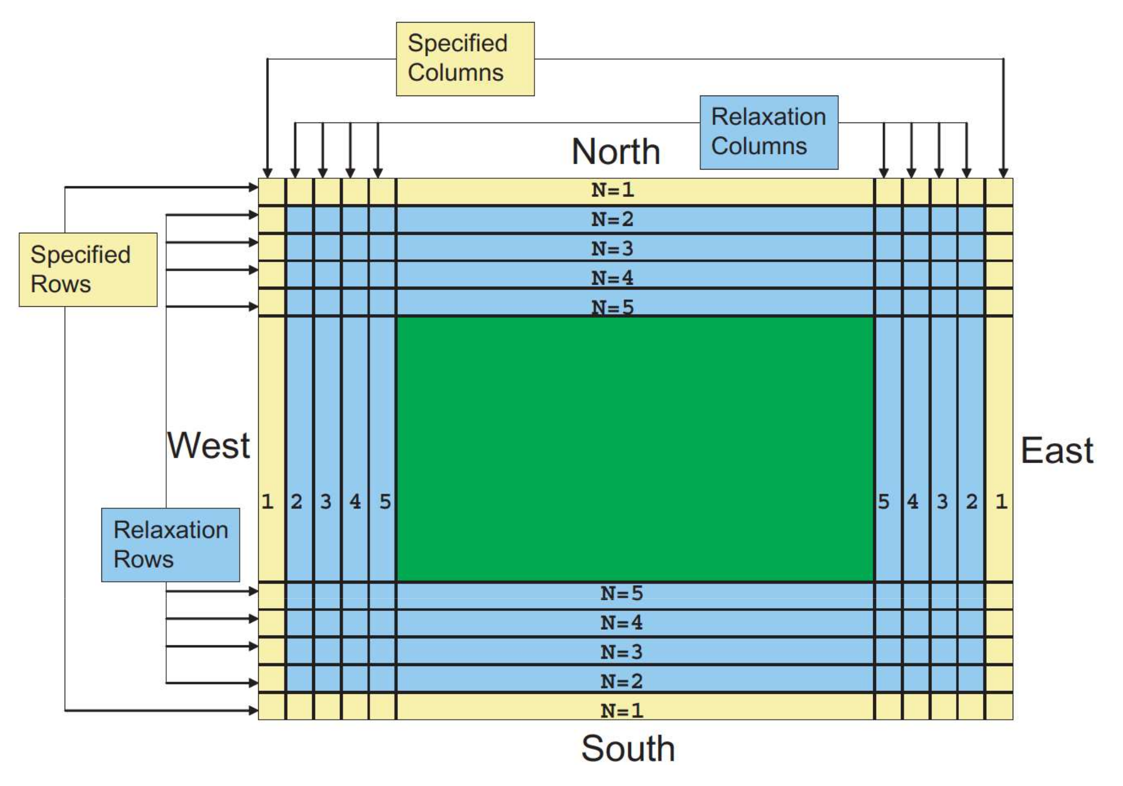
Real Domain BCs
When using real lateral boundary conditions, time-dependent observation data is read
from a file. In ERF, the observation (BDY) data is utilized to nudge the solution state towards
the observation data in the interior of the domain. We explicitly note that the wall normal
velocity on a domain boundary are set to the observational data and the RHS for these points
is assigned the BDY tendency. The user may specify (in the inputs file) the total
width of the interior boundary region with erf.real_width = <Int> (yellow + blue).
The real BCs are only imposed for \(\psi = \left\{ \theta; \; q_v; \; u; \; v \right\}\).
|
Image taken from Skamarock et al. (2021) |
To nudge the state data towards the observation data, we add a source term (\(G\)) to the RHS (\(F\)) of the governing equations:
where \(A\) is specified with erf.bdy_nudge_factor (defaults to 10.0),
\(\psi^{*}\) is the state variable at the current RK stage, \(\psi^{BDY}\) is
the temporal interpolation of the observational data, and \(\xi\) is a linear coordinate
that is 1 at the domain boundary and 0 at the edge of the nudge region.
For turbulent inflow perturbations, including the erf.perturbation_type options and
their placement on level subdomains, see Inflow Turbulence Generation.
ERF Boundary Data Files
For real lateral boundary conditions, init_type of metgrid or wrfinput, ERF can
write lateral boundary data to an AMReX-native file during initialization. The file name is
configurable with erf.erfbdy_file (default "erfbdy"). Use of the the erfbdy file is
mandatory for init_type of metgrid, but can be optionally disabled for init_type
of wrfinput with erf.write_erfbdy = false so that the boundary data is processed
as-needed during time integration.