Inflow Turbulence Generation
ERF provides the capability to apply a perturbation zone at the inflow boundary to
mechanically trip turbulence within the domain. The current version of the turbulence
generation techniques allows for x and y (horizontal) direction perturbations.
In Figure 2, as the bulk flow passes through the buoyant region, it becomes perturbed.
This perturbation, combined with a short development fetch, quickly leads to the
evolution of turbulence.
|
Image taken from DeLeon et al. (2018) |
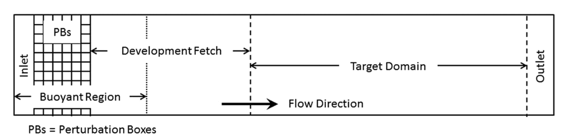
Four different types of perturbation methods are currently available,
source, direct, CPM, and CPM_W. The first two methods use the formulation
introduced by DeLeon et al. (2018) and are referred to as the box perturbation
method. The source option applies the perturbation amplitude range,
\(\pm \Phi_{PB}\), to each cell within the perturbation box as a source term.
The direct option uses the same rate but adds it, multiplied by the time step,
directly to the \(\rho \theta\) field at the start of every time step. Both
options add the same total perturbation over one update interval. The following
describes the theory of the box perturbation method:
The perturbation update interval of the individual perturbation box is determined by,
The change in the perturbation amplitude is defined as,
The current implementation supports lateral boundary perturbations, specified by
erf.perturbation_direction, where the six integer inputs represent perturbations
applied at the west, south, bottom, east, north, and top faces, respectively.
Note that while the top and bottom options are included, triggering either option
will abort the program.
At level 0, the perturbation boxes are placed inward from the corresponding domain face. On refined levels, ERF places perturbation boxes inward from the corresponding face of each subdomain on that level. In other words, each subdomain at a level is treated as its own local rectangular “domain” for the purpose of positioning perturbation boxes.
The current implementation assumes that every subdomain on a level where perturbations are enabled is rectangular and completely covered by grids at that level. If perturbations are requested on a level and any subdomain on that level is not rectangular, ERF will abort with an error.
In addition to the direction of perturbation, the flow perturbation method requires
the dimensions of an individual box, specified through erf.perturbation_box_dims,
with three integer inputs representing \({Nx}_{pb}\), \({Ny}_{pb}\), and
\({Nz}_{pb}\), respectively. Following the guidance of Ma and Senocak (2023),
the general rule of thumb is to use \(H_{PB} = 1/8 \delta\) as the height of
the perturbation box, where \(\delta\) is the boundary layer height. The length
of the box in the x-direction should be \(L_{PB} = 2H_{PB}\). Depending on the
direction of the bulk flow, the width of the box in the y-direction should be
defined as \(W_{PB} = L_{PB} \tan{(\theta_{inflow})}\). The current
implementation only accepts integer entries. Therefore, considering the domain size
and mesh resolution, the dimensions of a single box can be determined.
The perturbation mode is selected with erf.perturbation_type. This input may be
specified either once for all levels or once per level, following the same
convention used by erf.les_type. For example, in a two-level run,
erf.perturbation_type = None source
disables perturbations on level 0 and enables source perturbations on level 1.
The remaining perturbation inputs shown below are currently shared by all active
perturbation levels.
Specification of the number of layers and the offset into the domain or subdomain
of the perturbation boxes can be made through erf.perturbation_layers and
erf.perturbation_offset, respectively. Below is an example of the required
input tags to set up a simulation with inflow perturbations.
erf.perturbation_type = "source"

erf.perturbation_direction = 1 0 0 0 0 0
erf.perturbation_box_dims = 8 8 4
erf.perturbation_layers = 3
erf.perturbation_offset = 5

erf.perturbation_nondimensional = 0.042
erf.perturbation_T_infinity = 300.0
#erf.perturbation_T_intensity = 0.1
The erf.perturbation_T_intensity tag can be turned on or off by providing a
value or commenting it out. When a value is provided (recommended 0.1-0.25 max),
a pseudo-gravity value is used (solved from the Richardson formulation) to
normalize the scales of the problem, and is represented as,
Using this pseudo-gravity value effectively negates the Richardson number formulation, and the temperature gradient becomes,
where \(T_{i}\) is the temperature intensity, and \(T_{\infty}\) is the background temperature.
While this generates quick turbulence, it should be used as a sanity check rather than a runtime strategy for turbulence generation, therefore it is not recommended. Additionally, a net-zero energy enforcement is applied over the perturbation boxes to ensure that the synthetic method does not introduce excess energy into the system at each iteration. Below, we provide a detailed description of the two different types of perturbation methods currently existing within ERF.
Examples are provided within Exec/RegTests/TurbulentInflow/ to set up a
turbulent open channel flow using inflow/outflow boundary conditions with the
aforementioned turbulent inflow generation technique to trigger turbulence
downstream.
Source type forcing
By ignoring the advection and diffusion effects in the transport equation, the amplitude of the perturbation can be made through a proportionality ratio between the update time and change in the box temperature,
and the perturbation amplitude is then computed through,
source type forcing can adopt the box perturbation method by having the
following inputs list.
erf.perturbation_type = "source"

erf.perturbation_direction = 1 0 0 0 0 0
erf.perturbation_box_dims = 8 8 4
erf.perturbation_layers = 3
erf.perturbation_offset = 5

erf.perturbation_nondimensional = 0.042 # Ri
erf.perturbation_T_infinity = 300.0
The box perturbation method (BPM) perturbs the temperature field \(\rho \theta\) in a volume (box) format. Each box computes a perturbation update time and amplitude, then independently updates at its respective update interval during runtime. A single perturbation amplitude is seen by the computational cells that fall within this box. A pseudo-random perturbation (that is, white noise) is applied over the range \([-\phi, +\phi]\) then introduced to the \(\rho \theta\) field via source term (\(F_{\rho \theta}\)). As temperature is transported and through the action of the subgrid-scale (SGS) filter for eddy viscosity, white-noise temperature perturbations become colored noise in the velocity field. Since the perturbation enters only as a source term, none is added to the initial state; the forcing starts with the first time step.
The perturbations do not depend on the domain decomposition, for every
erf.perturbation_type. A perturbation box’s mean velocity, update interval and
net-zero correction (and, for CPM, its single random value) are computed over
the whole box, whichever grid boxes and MPI ranks it spans. The random values are
hashed from the global cell index (or, where there is one value per box, the box
index) and the number of times the box has been updated. The seed is 1024 with
erf.fix_random_seed = 1, otherwise erf.random_seed if it is given, and 0
otherwise, so a run is repeatable unless the seed is changed.
Turbulence onset can be triggered by adjusting the size of the perturbation box, as the amplitude is heavily influenced by having the two-dimensional scales of the perturbation box in the denominator.
Direct type forcing
The direct method computes the same amplitude and update interval as the
source method, and differs only in how the perturbation is added. Instead of
entering the right-hand side as a source term, the perturbation is added to the
\(\rho \theta\) field before each time step as
where \(\Delta t\) is the current time step of the level. Since the increment
is scaled by the current time step, a box receives a total of
\(\Delta \overline{\phi}\) over one update interval \(t_p\) even when the
time step varies. As for the source method, no perturbation is added at the
initial time.
To activate the direct type forcing, set the following inputs list.
erf.perturbation_type = "direct"

erf.perturbation_direction = 1 0 0 0 0 0
erf.perturbation_box_dims = 16 16 8
erf.perturbation_layers = 3
erf.perturbation_offset = 5

erf.perturbation_nondimensional = 0.042 # Ri
erf.perturbation_T_infinity = 300.0
Cell Perturbation Method
The cell perturbation method (CPM) is an implementation of the CPM that is available in WRF ( Muñoz-Esparza et al. (2014), Muñoz-Esparza et al. (2015), Muñoz-Esparza and Kosović (2018) ). The numerical implementation is similar to the box perturbation method described above with a few notable differences. Most notably there are no white-noise perturbations within each box/cell. Instead, the stochastic amplitude is applied to all nodes within a box/cell. The perturbation amplitude is formulated as follows:
where \(U_g\) is the geostrophic wind speed and \(Ec\) is the Eckert
number. The geostrophic wind speed can be considered the large-scale forcing.
In manual mode, this value is prescribed by the user (erf.perturbation_Ug) and
should represent the wind speed above the boundary layer and in the free
atmosphere. Automatic mode instead samples the horizontal wind at 1.1 times the
edge-mean PBL height on a coarser level, as described below. Previous research
has shown the optimum Eckert number to be 0.2 to
quickly develop turbulence (Muñoz-Esparza and Kosović (2018)).
CPM and CPM_W use a shared refresh interval per level by default, as described
under Uniform refresh for CPM and CPM_W below. With
erf.perturbation_uniform_refresh = false, each box retains its own
advective update interval:
where \(\langle \theta(z) \rangle_{PB}\) is the local wind direction and \(\langle U(z) \rangle_{PB}\) is the local wind speed of the box/cell. This per-box mode also retains the existing plus/minus 10% timing variation.
Below is an example of the input tags necessary for a simulation with CPM:
erf.perturbation_type = "CPM"

erf.perturbation_direction = 1 0 0 0 0 0
erf.perturbation_box_dims = 8 8 3
erf.perturbation_layers = 3
erf.perturbation_offset = 5

erf.perturbation_Ug = 10.0

erf.perturbation_klo = 1
erf.perturbation_khi = 40
Best practices are to set \({Nx}_{pb}=8\), \({Ny}_{pb}=8\), and
\({Nz}_{pb}=3\) regardless of the physical size of the boxes/cells and to set
erf.perturbation_layers = 3. The user can also specify the vertical extent of
the perturbation region using erf.perturbation_klo and erf.perturbation_khi.
For example, if the user would like to only perturb the atmospheric boundary layer up
to a specified inversion height, they can use erf.perturbation_khi to limit how
high the perturbations extend. Best practice is to specify erf.perturbation_klo = 1
to prevent any unphysical interactions with the bottom boundary conditions. If the user
does not specify the perturbation extents, the perturbation region will extend the entire
vertical column.
An example using CPM with a stable atmospheric boundary layer inflow setup is
available in Exec/RegTests/TurbulentInflow/.
A modified version of CPM is also available where the user can specify vertical velocity perturbations.
This pathway can be specified using erf.perturbation_type = "CPM_W". The user can specify the range
for the vertical velocity perturbations using erf.perturbation_w_amp. For example, if the user
specifies erf.perturbation_w_amp = 1.0, the range of the vertical velocity perturbations will be
[-1, 1].
Below is an example of the input tags to utilize the vertical velocity perturbation modification of CPM
with an example also in Exec/RegTests/TurbulentInflow/:
erf.perturbation_type = "CPM_W"

erf.perturbation_direction = 1 0 0 0 0 0
erf.perturbation_box_dims = 8 8 3
erf.perturbation_layers = 3
erf.perturbation_offset = 5

erf.perturbation_w_amp = 1.5

erf.perturbation_klo = 1
erf.perturbation_khi = 40
Uniform refresh for CPM and CPM_W
erf.perturbation_uniform_refresh = true is the default for CPM and CPM_W.
All perturbation boxes on a level draw new random values together, using one
advective interval for that level. Separate levels have separate clocks.
The source and direct methods retain their per-box timing.
Set the flag to false to restore the previous CPM/CPM_W timing.
Input |
Default |
Meaning |
|---|---|---|
|
|
Use one refresh clock per CPM/CPM_W level, without per-box timing jitter. |
|
|
Wind-sampling height in meters AGL when |
|
|
Seconds between timing-wind samples when |
In automatic mode, the timing wind is sampled at 0.05 times each active
edge’s mean PBL height, in meters AGL. ERF chooses the finest coarser level
covering that height along the entire edge, starting with the immediate parent.
These winds are resampled with the other automatic controls, using
perturbation_auto_period (600 seconds by default).
In idealized or other manual cases, the timing wind comes from the receiving
level at perturbation_refresh_height. This also works on level 0 and does
not require a PBL diagnostic. Sampling uses a one-column strip along each
configured lateral perturbation edge, inset by perturbation_offset.
The nest must reach the ground and contain the sampling height along those
edges. The height is independent of perturbation_klo and
perturbation_khi. Wind interpolation and averaging use the same method as
the automatic wind sampler.
Let \(\bar u_e,\bar v_e\) be the horizontally averaged wind components at the sampling height on edge \(e\). The shared refresh interval is
This retains the existing CPM box-size, layer-count and wind-angle scaling; the fastest sampled edge determines the interval for the whole level. For example, 800 m boxes, three layers and \(S=5\) m/s give 480 seconds. The first refresh occurs on the first advance, including for a delayed nest. Later refreshes occur on the first time step at or after the shared deadline, and the next deadline is measured from that refresh. Each wind-control update starts a new shared cycle immediately. Regrids and restarts initialize fresh clocks. When all sampled winds are calm, no increments are applied; wind sampling continues on its control period so perturbations can resume.
Between refreshes, ERF skips perturbation-box scans, forcing-field clearing,
and perturbation application. Stored increments are applied only on a refresh
step. CPM still determines its amplitude from perturbation_Ug or the
automatic wind at 1.1 times PBLH, and CPM_W still uses perturbation_w_amp.
The near-surface timing wind does not change either amplitude formula.
For an idealized case, the defaults can be written explicitly as:
erf.perturbation_uniform_refresh = true
erf.perturbation_refresh_height = 20.0
erf.perturbation_refresh_wind_period = 600.0
Automatic perturbations on LES nests
Set erf.perturbation_auto = true to obtain the active inflow edges and
advective wind scale from each nest’s immediate parent, and the height limit
from its finest ancestor using a PBL scheme. When no ancestor uses a PBL scheme,
the height comes from the nearest coarser three-dimensional LES level’s
surface-layer diagnostic. Automatic mode defaults
to true for erf.init_type = WRFInput or Metgrid and false for
other initialization types. An explicit erf.perturbation_auto = false
retains the manual controls described above. This option works with source,
direct, CPM and CPM_W. A perturbation method must still be selected
with erf.perturbation_type; its default remains None.
In automatic mode, ERF enables the requested perturbation type only on refined
levels using a three-dimensional LES closure (Smagorinsky or Deardorff) without
a PBL scheme. Level 0, PBL levels, RANS levels and Smagorinsky2D levels receive
no perturbations. An explicit None in the per-level perturbation-type list
still disables that level. The immediate parent may use a PBL scheme or be
another LES level. For the PBL height, ERF searches from that parent toward
level 0 and selects the first level with a PBL scheme. For example, with a
PBL scheme on level 0 and LES on levels 1 and 2, both LES levels use level 0’s
PBL height; level 1 samples level 0’s winds, while level 2 samples level 1’s
winds. If levels 0 and 1 both use PBL schemes, an LES level 2 instead uses
level 1’s PBL height.
When all levels use LES, level 1 uses level 0’s diagnosed PBL height and
level 2 uses level 1’s diagnostic. This uses most.pblh_calc = MYNN25 on
the bottom surface_layer boundary, independently of erf.pbl_type;
the LES closures remain unchanged. Automatic mode supplies this diagnostic
setting when it is not explicitly specified. A refined LES ancestor whose
grids do not cover the full vertical domain inherits the diagnostic from its
coarser level through the existing surface-layer machinery. An explicit
most.pblh_calc = none or a scheme-only diagnostic such as YSU cannot
supply the LES fallback; select MYNN25 in that case. Missing or invalid
heights remain errors.
For example, add the following to a two-level case with a YSU parent and a Deardorff nest. The case must also have the surface-layer inputs required by its PBL scheme:
erf.les_type = None Deardorff
erf.pbl_type = YSU None
erf.perturbation_type = CPM
erf.perturbation_auto = true
erf.perturbation_auto_period = 600.0
erf.perturbation_auto_pbl_fraction = 0.9

erf.perturbation_box_dims = 8 8 3
erf.perturbation_layers = 3
erf.perturbation_offset = 5
The automatic controls are:
Input |
Default |
Meaning |
|---|---|---|
|
Depends on initialization |
Enable parent controls on eligible LES nests, using a PBL ancestor’s height or an LES diagnostic fallback; defaults to |
|
|
Seconds between updates of edges, height and wind scale; must be positive. |
|
|
Fraction of the selected ancestor’s PBL height; must be greater than zero and at most one. |
At the first advance of a nest, ERF samples the latest available parent state.
For each lateral edge of each rectangular subdomain, it samples one parent
column in width along that edge. Each parent column uses the PBL height of the
cell containing it on the selected ancestor. This mapping uses the cumulative
horizontal refinement ratio and retains the ancestor’s height in meters AGL.
It averages the horizontal wind components over the lower
perturbation_auto_pbl_fraction of that height, weighting
by the vertical cell thickness inside that layer. If the parent grids end
below that height, the wind average uses the available part of the layer.
Wind components are in the simulation’s grid directions. A positive mean
u selects the west edge and a negative mean u selects the east edge;
positive and negative mean v select the south and north edges, respectively.
Each edge uses its own average, so opposing edges can both be active if the
parent winds vary spatially. Periodic physical edges, walls and symmetry faces
are excluded. Internal coarse/fine edges remain eligible.
The height cutoff for an edge is the specified fraction of the ancestor PBL
height averaged over the sampled parent columns: by default, 90% of this edge
mean. Each column contributes once to the arithmetic mean. This produces one
uniform cutoff in meters AGL along each edge and throughout its perturbation
layers; it does not vary with the PBL height at individual columns. Different
edges may have different means. Perturbations are applied only where the sample
point lies above local ground and at or below this cutoff: cell centers for thermal perturbations and
vertical-velocity faces for CPM_W. Thus the cutoff follows the nest’s local
terrain and can cut through a perturbation box. Shared corners receive one
increment; they are active if either adjoining edge permits perturbations.
Where a box intersects two active edges, the larger lower-PBL wind speed sets
its per-box refresh interval (when used) and its source/direct amplitude. For CPM, the
larger above-PBL wind scale sets its amplitude.
For CPM, ERF obtains Ug by sampling horizontal wind at 1.1 times the
edge-mean PBL height, in meters AGL. It first tries the immediate parent and
then successively coarser levels, choosing the finest ancestor whose grids
cover that height in every sampled column along the edge. The PBL height still
comes from the selected PBL or LES ancestor. If no coarser level covers
the target height, automatic CPM stops with an error.
On the selected level, ERF linearly interpolates cell-centered u and v
to the target height in each column, averages each component along the edge,
and sets Ug = sqrt(mean(u)^2 + mean(v)^2). It uses the nearest cell center
within the bottom or top half-cell, and never extrapolates outside the
available grid. This above-PBL wind estimate replaces perturbation_Ug in
the CPM amplitude formula. It is independent of the lower-PBL wind used for
inflow selection and advective refresh timing. source and direct retain
the lower-PBL parent wind for their existing amplitude and refresh formulas.
CPM_W retains perturbation_w_amp for its vertical-velocity amplitude.
The controls are initialized on the first advance of each nest, including nests
created later in the simulation. They use the latest available ancestor PBLH
and winds. Timing uses seconds elapsed from the simulation’s start. Regridding
or restarting also forces a fresh control update on the next advance.
Afterward, the controls are recomputed on the first nest time step at or after
the update period has elapsed since the previous control update (600 seconds
by default).
Between control updates, CPM/CPM_W boxes draw new random values on their shared
clock by default; with uniform refresh disabled, they use their individual
advective intervals. The source and direct methods also retain their
individual intervals. At a control update, ERF
clears the previous forcing and regenerates it under the new controls. Calm
edges are disabled and can become active at a later update. This clears stored
forcing; perturbations already advected into the solution continue to evolve.
perturbation_box_dims, perturbation_layers and perturbation_offset
remain required. Layers must be positive, and the offset must leave space
inside the nest. Dimensions and offsets are specified in cells at each level.
perturbation_direction, perturbation_Ug, perturbation_klo and
perturbation_khi do not control the automatic regions. Thermal perturbations
may include the lowest cell center; CPM_W excludes the ground face.
The selected ancestor’s height comes from its bottom surface_layer
diagnostic, or from native SHOC’s PBL-height diagnostic. When the bottom surface
layer has no explicit most.pblh_calc input, automatic mode supplies
MYNN25. The MYNN diagnostic always uses heights above local ground,
including its near-surface temperature scan
and TKE blending. YSU, YSUNew and MRF write their scheme’s height to the surface
layer as they advance. An explicit most.pblh_calc setting is respected in
the bottom face’s input namespace; it must provide a valid height on the
selected ancestor. The MYNN25 diagnostic can run on LES fields: it combines
a virtual-potential-temperature increase criterion with a TKE criterion.
For Deardorff LES, the stored TKE is subgrid TKE; this diagnostic does not add
resolved velocity variance. A diagnosed height of zero contributes zero to the edge
mean and provides no depth for the wind average. Missing or uninitialized
heights cause an error when the controls are updated.
Automatic mode currently supports rectangular nests that reach the ground, on flat, stretched or fitted-terrain meshes. Immersed-forcing terrain and embedded boundary terrain are not supported. The finest cells and their parent cells need not have the same vertical spacing or domain height. Regridding, delayed nest creation and restarting reset the control timer and recompute the controls at the next advance; random refresh counters are not checkpointed, so a restart does not reproduce an uninterrupted random sequence.
Set erf.v = 1 to log each control update’s time, wind-parent level
(parent), PBL-height source level (pbl_level), source type
(pblh_source = PBL or LES), edge, inflow selection,
mean wind and height cutoff in meters AGL.
For CPM, the log also reports the wind source level (Ug_level), target
height (Ug_height_agl), and sampled speed (Ug). An inactive edge has
Ug_level = -1 because it does not need an amplitude sample.