Meshing
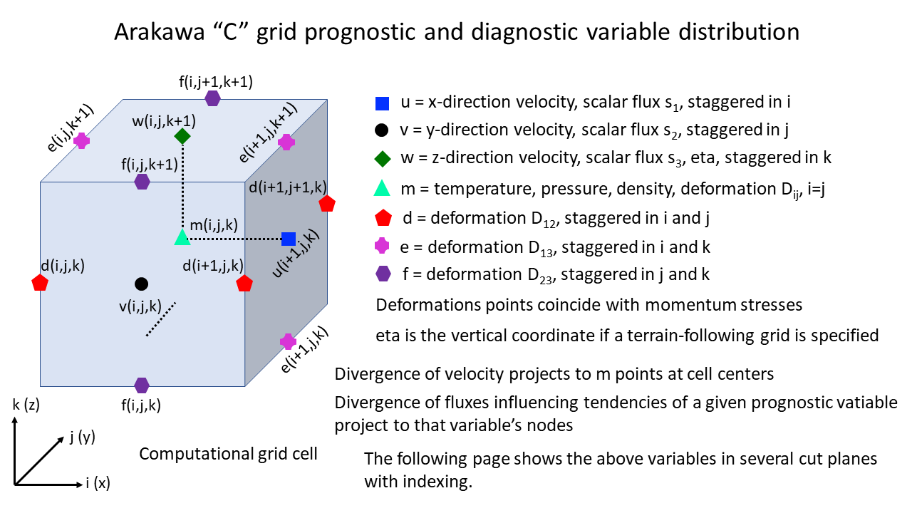
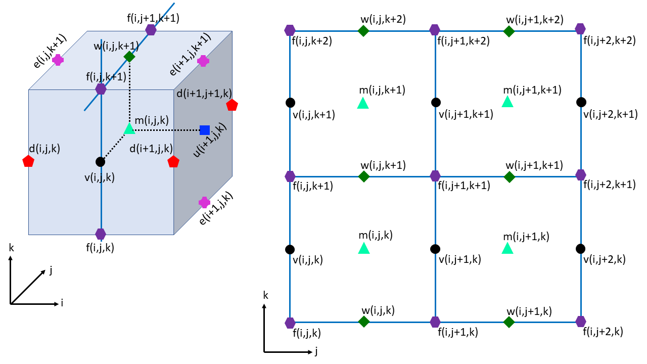
The spatial discretization in ERF uses the classic Arakawa C-grid with scalar quantities at cell centers and normal velocities at cell faces. Simulations over complex topography have the option to use a terrain-following, height-based vertical coordinate. When terrain-following coordinates are used, the surface topography at nodes (cell corners) is specified either analytically or through parsing a text file; all metric terms derive from this quantity.
See WoA for an example of a terrain-fitted grid; this one follows the Witch of Agnesi profile.
As in many atmospheric modeling codes, variable mesh spacing in the vertical direction is allowed with or without terrain. The heights of each level can be parsed from a text file as “z levels” (as in WRF), or calculated at run-time given an initial mesh spacing at the bottom surface and a specified growth rate. In the presence of non-flat terrain, the mesh is modified so that it fits the specified terrain at the bottom of the computational domain, and relaxes to flat at the top of the domain. Three approaches to this are offered in ERF: Basic Terrain Following (BTF), in which the influence of the terrain decreases linearly with height; Smoothed Terrain Following (STF), in which small-scale terrain structures are progressively smoothed out of the coordinate system as height increases; or Sullivan Terrain Following (Sullivan), in which the influence of the terrain decreases with the cube of height. Additionally, ERF includes the capability to apply several common isotropic map projections (e.g., Lambert Conformal, Mercator); see Map Factors (Dry) for more details.