Inflow Turbulence Generation

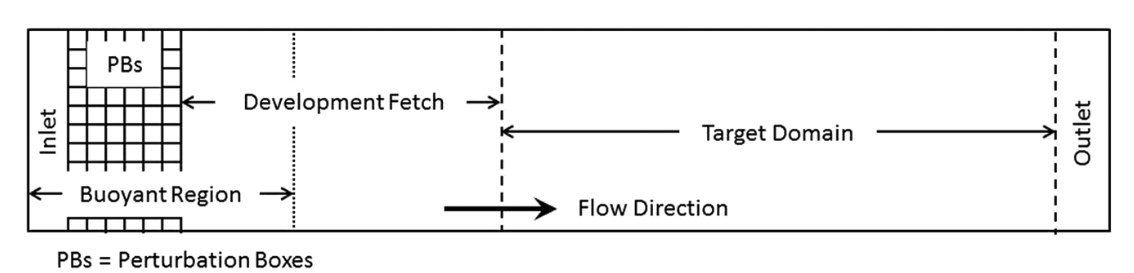
ERF provides the capability to apply a perturbation zone at the inflow boundary to mechanically trip turbulence within the domain. The current version of the turbulence generation techniques allows for x and y (horizontal) direction perturbations. In Figure 2, as the bulk flow passes through the buoyant region, it becomes perturbed. This perturbation, combined with a short development fetch, quickly leads to the evolution of turbulence.

9 Box perturbation method

Image taken from DeLeon et al. (2018)

Three different types of perturbation methods are currently available, source, direct, and CPM. The first two methods use the formulation introduced by DeLeon et al. (2018) and are referred to as the box perturbation method. The source option applies the perturbation amplitude range, \(\pm \Phi_{PB}\), to each cell within the perturbation box as a source term. Conversely, the direct option applies the calculated temperature difference directly onto the \(\rho \theta\) field. We note that while both methods effectively generate turbulence downstream, the latter approach is more unstable and requires more fine tuning. The following describes the theory of the box perturbation method:

The perturbation update interval of the individual perturbation box is determined by,

\[\frac{t_p \langle U(z) \rangle_{PB}}{D_{PB}} = 1,\]

The change in the perturbation amplitude is defined as,

\[{Ri}_{PB} = \frac{g \beta \Delta \overline{\phi} H_{PB}}{{\langle U(z) \rangle}^2_{PB}}.\]

The current implementation supports lateral boundary perturbations, specified by erf.perturbation_direction, where the six integer inputs represent perturbations applied at the west, south, bottom, east, north, and top faces, respectively. Note that while the top and bottom options are included, triggering either option will abort the program.

At level 0, the perturbation boxes are placed inward from the corresponding domain face. On refined levels, ERF places perturbation boxes inward from the corresponding face of each subdomain on that level. In other words, each subdomain at a level is treated as its own local rectangular “domain” for the purpose of positioning perturbation boxes.

The current implementation assumes that every subdomain on a level where perturbations are enabled is rectangular and completely covered by grids at that level. If perturbations are requested on a level and any subdomain on that level is not rectangular, ERF will abort with an error.

In addition to the direction of perturbation, the flow perturbation method requires the dimensions of an individual box, specified through erf.perturbation_box_dims, with three integer inputs representing \({Nx}_{pb}\), \({Ny}_{pb}\), and \({Nz}_{pb}\), respectively. Following the guidance of Ma and Senocak (2023), the general rule of thumb is to use \(H_{PB} = 1/8 \delta\) as the height of the perturbation box, where \(\delta\) is the boundary layer height. The length of the box in the x-direction should be \(L_{PB} = 2H_{PB}\). Depending on the direction of the bulk flow, the width of the box in the y-direction should be defined as \(W_{PB} = L_{PB} \tan{(\theta_{inflow})}\). The current implementation only accepts integer entries. Therefore, considering the domain size and mesh resolution, the dimensions of a single box can be determined.

The perturbation mode is selected with erf.perturbation_type. This input may be specified either once for all levels or once per level, following the same convention used by erf.les_type. For example, in a two-level run,

erf.perturbation_type = None source

disables perturbations on level 0 and enables source perturbations on level 1. The remaining perturbation inputs shown below are currently shared by all active perturbation levels.

Specification of the number of layers and the offset into the domain or subdomain of the perturbation boxes can be made through erf.perturbation_layers and erf.perturbation_offset, respectively. Below is an example of the required input tags to set up a simulation with inflow perturbations.

erf.perturbation_type = "source"

erf.perturbation_direction = 1 0 0 0 0 0
erf.perturbation_box_dims = 8 8 4
erf.perturbation_layers = 3
erf.perturbation_offset = 5

erf.perturbation_nondimensional = 0.042
erf.perturbation_T_infinity = 300.0
#erf.perturbation_T_intensity = 0.1

The erf.perturbation_T_intensity tag can be turned on or off by providing a value or commenting it out. When a value is provided (recommended 0.1-0.25 max), a pseudo-gravity value is used (solved from the Richardson formulation) to normalize the scales of the problem, and is represented as,

\[g = \frac{{Ri}_{PB} {\langle U(z) \rangle}^2_{PB}}{\beta \Delta \phi H_{pb}}.\]

Using this pseudo-gravity value effectively negates the Richardson number formulation, and the temperature gradient becomes,

\[\Delta \phi = T_{i} T_{\infty},\]

where \(T_{i}\) is the temperature intensity, and \(T_{\infty}\) is the background temperature.

While this generates quick turbulence, it should be used as a sanity check rather than a runtime strategy for turbulence generation, therefore it is not recommended. Additionally, a net-zero energy enforcement is applied over the perturbation boxes to ensure that the synthetic method does not introduce excess energy into the system at each iteration. Below, we provide a detailed description of the two different types of perturbation methods currently existing within ERF.

Examples are provided within Exec/RegTests/TurbulentInflow/ to set up a turbulent open channel flow using inflow/outflow boundary conditions with the aforementioned turbulent inflow generation technique to trigger turbulence downstream.

Source type forcing

By ignoring the advection and diffusion effects in the transport equation, the amplitude of the perturbation can be made through a proportionality ratio between the update time and change in the box temperature,

\[\Phi_{PB} \propto \frac{\Delta \overline{\phi}}{t_p}\]

and the perturbation amplitude is then computed through,

\[\Phi_{PB} = \frac{Ri_{PB} {\langle U(z) \rangle}^2_{PB}}{g \beta D_{PB} H_{PB}}.\]

source type forcing can adopt the box perturbation method by having the following inputs list.

erf.perturbation_type = "source"

erf.perturbation_direction = 1 0 0 0 0 0
erf.perturbation_box_dims = 8 8 4
erf.perturbation_layers = 3
erf.perturbation_offset = 5

erf.perturbation_nondimensional = 0.042 # Ri
erf.perturbation_T_infinity = 300.0

The box perturbation method (BPM) perturbs the temperature field \(\rho \theta\) in a volume (box) format. Each box computes a perturbation update time and amplitude, then independently updates at its respective update interval during runtime. A single perturbation amplitude is seen by the computational cells that fall within this box. A pseudo-random perturbation (that is, white noise) is applied over the range \([-\phi, +\phi]\) then introduced to the \(\rho \theta\) field via source term (\(F_{\rho \theta}\)). As temperature is transported and through the action of the subgrid-scale (SGS) filter for eddy viscosity, white-noise temperature perturbations become colored noise in the velocity field.

Using the source term to perturb the momentum field through buoyancy coupling requires more time compared to the direct perturbation method. Turbulence onset can be triggered by adjusting the size of the perturbation box, as the amplitude is heavily influenced by having the two-dimensional scales of the perturbation box in the denominator.

Direct type forcing

The direct method can also be used to effectively trip turbulence into the domain. Minute differences exist between the direct and source method, with the primary one being the perturbation amplitude is directly solved from the Richardson number relationship as,

\[\Phi_{PB} = \frac{Ri_{PB} {\langle U(z) \rangle}^2_{PB}}{g \beta H_{PB}}.\]

To activate the direct type forcing, set the following inputs list.

erf.perturbation_type = "direct"

erf.perturbation_direction = 1 0 0 0 0 0
erf.perturbation_box_dims = 16 16 8
erf.perturbation_layers = 3
erf.perturbation_offset = 5

erf.perturbation_nondimensional = 0.042 # Ri
erf.perturbation_T_infinity = 300.0

We want to note that the direct perturbation method is sensitive to the temperature amplitude computed through the equation above, and is subject to crash the simulation when this amplitude is too large.

Cell Perturbation Method

The cell perturbation method (CPM) is an implementation of the CPM that is available in WRF ( Muñoz-Esparza et al. (2014), Muñoz-Esparza et al. (2015), Muñoz-Esparza and Kosović (2018) ). The numerical implementation is similar to the box perturbation method described above with a few notable differences. Most notably there are no white-noise perturbations within each box/cell. Instead, the stochastic amplitude is applied to all nodes within a box/cell. The perturbation amplitude is formulated as follows:

\[\Phi_{PB} = \frac{U_g^2}{c_p Ec},\]

where \(U_g\) is the geostrophic wind speed and \(Ec\) is the Eckert number. The geostrophic wind speed can be considered the large-scale forcing. Currently, this value is prescribed by the user (erf.perturbation_Ug) and should represent the wind speed above the boundary layer and in the free atmosphere. In the future, the geostrophic wind will be automatically calculated within the code. Previous research has shown the optimum Eckert number to be 0.2 to quickly develop turbulence (Muñoz-Esparza and Kosović (2018)).

The perturbation update interval depends on the advective time scale for flow through the perturbation boxes/cells:

\[t_p = \frac{L_{PB} \cdot \text{num_layers}}{\cos{\left(\langle \theta(z) \rangle_{PB} \right)} \langle U(z) \rangle_{PB}},\]

where \(\langle \theta(z) \rangle_{PB}\) is the local wind direction and \(\langle U(z) \rangle_{PB}\) is the local wind speed of the box/cell.

Below is an example of the input tags necessary for a simulation with CPM:

erf.perturbation_type = "CPM"

erf.perturbation_direction = 1 0 0 0 0 0
erf.perturbation_box_dims = 8 8 3
erf.perturbation_layers = 3
erf.perturbation_offset = 5

erf.perturbation_Ug = 10.0

Best practices are to set \({Nx}_{pb}=8\), \({Ny}_{pb}=8\), and \({Nz}_{pb}=3\) regardless of the physical size of the boxes/cells and to set erf.perturbation_layers = 3.

An example using CPM with a stable atmospheric boundary layer inflow setup is available in Exec/RegTests/TurbulentInflow/.